Mikles J., Fikar M. Process Modelling, Identification, and Control
Подождите немного. Документ загружается.


3.2 State-Space Process Models 77
Asymptotic stability: If a positive definite function V (x) can be chosen
such that
dV
dt
=
∂V
∂x
T
f(x) < 0, x = 0 (3.77)
then the system is asymptotically stable in origin.
Asymptotic stability in large: If the conditions of asymptotic stability are
satisfied for all x and if V (x) →∞for x→∞then the system is asymp-
totically stable by large in origin.
There is no general procedure for the construction of the Lyapunov func-
tion. If such a function exists then it is not unique. Often it is chosen in the
form
V (x)=
n
k=1
n
r=1
K
rk
x
k
x
r
(3.78)
K
rk
are real constants, K
rk
= K
kr
so (3.78) can be written as
V (x)=x
T
Kx (3.79)
and K is symmetric matrix. V (x) is positive definite if and only if the deter-
minants
K
11
,
K
11
,K
12
K
21
,K
22
,
K
11
,K
12
,K
13
K
21
,K
22
,K
23
K
31
,K
32
,K
33
,... (3.80)
are greater than zero.
Asymptotic stability of linear systems: Linear system
dx(t)
dt
= Ax(t) (3.81)
is asymptotically stable (in large) if and only if one of the following properties
is valid:
1. Lyapunov equation
A
T
K + KA = −μ (3.82)
where μ is any symmetric positive definite matrix, has a unique positive
definite symmetric solution K.
2. all eigenvalues of system matrix A, i.e. all roots of characteristic polyno-
mial det(sI −A) have negative real parts.
Proof : We prove only the sufficient part of 1. Consider the Lyapunov func-
tion of the form
V (x)=x
T
Kx (3.83)

78 3 Analysis of Process Models
if K is a positive definite then
V (x) > 0 , x = 0 (3.84)
V (0) = 0 (3.85)
and for dV/dt holds
dV (x)
dt
=
dx
dt
T
Kx + x
T
K
dx
dt
(3.86)
Substituting dx/dt from Eq. (3.81) yields
dV (x)
dt
= x
T
A
T
Kx + x
T
KAx (3.87)
dV (x)
dt
= x
T
(A
T
K + KA)x (3.88)
Applying (3.82) we get
dV (x)
dt
= −x
T
μx (3.89)
and because μ is a positive definite matrix then
dV (x)
dt
< 0 (3.90)
for all x = 0 and the system is asymptotically stable in origin. As the Lya-
punov function can be written as
V (x)=x
2
(3.91)
and therefore
V (x) →∞ for x→∞ (3.92)
The corresponding norm is defined as (x
T
Kx)
1/2
. It can easily be shown that
K exists and all conditions of the theorem on asymptotic stability by large in
origin are fulfilled. The second part of the proof - necessity - is much harder
to prove.
The choice of μ for computations is usually
μ = I (3.93)
Controllability of Continuous-Time Systems
The concept of controllability together with observability is of fundamental
importance in theory of automatic control.
Definition of controllability of linear system

3.2 State-Space Process Models 79
dx(t)
dt
= A(t)x(t)+B(t)u(t) (3.94)
is as follows: A state x(t
0
) = 0 of the system (3.94) is control lable if the
system can be driven from this state to state x(t
1
)=0 by applying suitable
u(t) within finite time t
1
− t
0
,t∈ [t
0
,t
1
].
If every state is controllable then the system is completely controllable.
Definition of reachable of linear systems: A state x(t
1
) of the system (3.94)
is reachable if the system can be driven from the state x(t
0
)=0 to x(t
1
)by
applying suitable u(t) within finite time t
1
− t
0
,t∈ [t
0
,t
1
].
If every state is reachable then the system is completely reachable.
For linear systems with constant coefficients (linear time invariant sys-
tems) are all reachable states controllable and it is sufficient to speak about
controllability. Often the definitions are simplified and we can speak that the
system is completely controllable (shortly controllable) if there exists such
u(t) that drives the system from the arbitrary initial state x(t
0
) to the final
state x(t
1
) within a finite time t
1
− t
0
,t∈ [t
0
,t
1
].
Theorem (Controllability of linear continuous systems with constant coef-
ficients): The system
dx(t)
dt
= Ax(t)+Bu(t) (3.95)
y(t)=Cx(t) (3.96)
is completely controllable if and only if rank of controllability matrix Q
c
is
equal to n. Q
c
[n ×nm] is defined as
Q
c
=(BABA
2
B ...A
n−1
B) (3.97)
where n is the dimension of the vector x and m is the dimension of the vector
u.
Proof : We prove only the “if” part. Solution of the Eq. (3.95) with initial
condition x(t
0
)is
x(t)=e
At
x(t
0
)+
t
0
e
A(t−τ)
Bu(τ )dτ (3.98)
For t = t
1
follows
x(t
1
)=e
At
1
x(t
0
)+e
At
1
t
1
0
e
−Aτ
Bu(τ )dτ (3.99)
The function e
−Aτ
can be rewritten with the aid of the Cayley-Hamilton
theorem as
e
−Aτ
= k
0
(τ)I + k
1
(τ)A + k
2
(τ)A
2
+ ···+ k
n−1
(τ)A
n−1
(3.100)
Substituting for e
−Aτ
from (3.100) into (3.99) yields
80 3 Analysis of Process Models
x(t
1
)=e
At
1
x(t
0
)+e
At
1
t
1
0
k
0
(τ)B + k
1
(τ)AB +
+k
2
(τ)A
2
B + ···+ k
n−1
(τ)A
n−1
B
u(τ)dτ (3.101)
or
x(t
1
)=e
At
1
x(t
0
)+
+e
At
1
t
1
0
(BABA
2
B ...A
n−1
B) ×
×
⎛
⎜
⎜
⎜
⎜
⎜
⎝
k
0
(τ)u(τ )
k
1
(τ)u(τ )
k
2
(τ)u(τ )
.
.
.
k
n−1
(τ)u(τ )
⎞
⎟
⎟
⎟
⎟
⎟
⎠
dτ (3.102)
Complete controllability means that for all x(t
0
) = 0 there exists a finite
time t
1
− t
0
and suitable u(t) such that
−x(t
0
)=(BABA
2
B ...A
n−1
B)
t
1
0
⎛
⎜
⎜
⎜
⎜
⎜
⎝
k
0
(τ)u(τ )
k
1
(τ)u(τ )
k
2
(τ)u(τ )
.
.
.
k
n−1
(τ)u(τ )
⎞
⎟
⎟
⎟
⎟
⎟
⎠
dτ (3.103)
From this equation follows that any vector −x(t
0
) can be expressed as a linear
combination of the columns of Q
c
. The system is controllable if the integrand
in (3.102) allows the influence of u to reach all the states x. Hence complete
controllability is equivalent to the condition of rank of Q
c
being equal to n.
The controllability theorem enables a simple check of system controllability
with regard to x. The test with regard to y can be derived analogously and
is given below.
Theorem (Output controllability of linear systems with constant coeffi-
cients): The system output y of (3.95), (3.96) is completely controllable if
and only if the rank of controllability matrix Q
y
c
[r × nm] is equal to r (with
r being dimension of the output vector) where
Q
y
c
=(CB CAB CA
2
B ...CA
n−1
B) (3.104)
We note that the controllability conditions are also valid for linear systems
with time-varying coefficients if A(t), B(t) are known functions of time. The
conditions for nonlinear systems are derived only for some special cases. For-
tunately, in the majority of practical cases, controllability of nonlinear systems
is satisfied if the corresponding linearised system is controllable.
Example 3.7: CSTR - controllability
Linearised state-space model of CSTR (see Example 2.6) is of the form
3.2 State-Space Process Models 81
dx
1
(t)
dt
= a
11
x
1
(t)+a
12
x
2
(t)
dx
2
(t)
dt
= a
21
x
1
(t)+a
22
x
2
(t)+b
21
u
1
(t)
or
dx(t)
dt
= Ax(t)+Bu
1
(t)
where
A =
a
11
a
12
a
21
a
22
, B =
0
b
21
The controllability matrix Q
c
is
Q
c
=(B|AB)=
0 a
12
b
21
b
21
a
22
b
21
and has rank equal to 2 and the system is completely controllable. It is
clear that this is valid for all steady-states and hence the corresponding
nonlinear model of the reactor is controllable.
Observability
States of a system are in the majority of cases measurable only partially or
they are nonmeasurable. Therefore it is not possible to realise a control that
assumes knowledge of state variables. In this connection a question arises
whether it is possible to determine state vector from output measurements. We
speak about observability and reconstructibility. To investigate observability,
only a free system can be considered.
Definition of observability: A state x(t
0
) of the system
dx(t)
dt
= A(t)x(t) (3.105)
y(t)=C(t)x(t) (3.106)
is observable if it can be determined from knowledge about y(t) within a finite
time t ∈ [t
0
,t
1
]. If every state x(t
0
) can be determined from the output vector
y(t) within arbitrary finite interval t ∈ [t
0
,t
1
] then the system is completely
observable.
Definition of reconstructibility : A state of system x(t
0
) is reconstructible
if it can be determined from knowledge about y(t) within a finite time
t ∈ [t
00
,t
0
]. If every state x(t
0
) can be determined from the output vector
y(t) within arbitrary finite interval t ∈ [t
00
,t
0
] then the system is completely
reconstructible.
Similarly as in the case of controllability and reachability, the terms observ-
ability of a system and reconstructibility of a system are used for simplicity.
For linear time-invariant systems, both terms are interchangeable.

82 3 Analysis of Process Models
Theorem: Observability of linear continuous systems with constant coeffi-
cients: The system
dx(t)
dt
= Ax(t) (3.107)
y(t)=Cx(t) (3.108)
is completely observable if and only if rank of observability matrix Q
o
is equal
to n. The matrix Q
o
[nr × n] is given as
Q
o
=
⎛
⎜
⎜
⎜
⎜
⎜
⎝
C
CA
CA
2
.
.
.
CA
n−1
⎞
⎟
⎟
⎟
⎟
⎟
⎠
(3.109)
Proof : We prove only the “if” part. Solution of the Eq. (3.107) is
x(t)=e
At
x(t
0
) (3.110)
According to the Cayley-Hamilton theorem, the function e
−At
can be written
as
e
−At
= k
0
(t)I + k
1
(t)A + k
2
(t)A
2
+ ···+ k
n−1
(t)A
n−1
(3.111)
Substituting Eq. (3.111) into (3.110) yields
x(t)=[k
0
(t)I + k
1
(t)A + k
2
(t)A
2
+ ···+ k
n−1
(t)A
n−1
]x(t
0
) (3.112)
Equation (3.108) now gives
y(t)=[k
0
(t)C +k
1
(t)CA+k
2
(t)CA
2
+···+k
n−1
(t)CA
n−1
]x(t
0
) (3.113)
or
x(t
0
)=
t
1
t
0
(k(t)Q
o
)
T
(k(t)Q
o
)dt
−1
t
1
t
0
(k(t)Q
o
)
T
y(t)dt (3.114)
where k(t)=[k
0
(t),k
1
(t),...,k
n−1
(t)].
If the system is observable, it must be possible to determine x(t
0
)from
(3.114). Hence the inverse of
t
1
t
0
(k(t)Q
o
)
T
(k(t)Q
o
)dt must exist and the ma-
trix
t
1
t
0
(k(t)Q
o
)
T
(k(t)Q
o
)dt = Q
o
T
t
1
t
0
(k
T
(t)k(t)dtQ
o
(3.115)
must be nonsingular. It can be shown that the matrix k
T
(t)k(t) is nonsingular
and observability is satisfied if and only if rank(Q
o
)=n.

3.2 State-Space Process Models 83
We note that observability and reconstructibility conditions for linear con-
tinuous systems with constant coefficients are the same.
Example 3.8: CSTR - observability
Consider the linearised model of CSTR from Example 2.6
dx
1
(t)
dt
= a
11
x
1
(t)+a
12
x
2
(t)
dx
2
(t)
dt
= a
21
x
1
(t)+a
22
x
2
(t)
y
1
(t)=x
2
(t)
The matrices A, C are
A =
a
11
a
12
a
21
a
22
, C =(0, 1)
and for Q
o
yields
Q
o
=
01
a
21
a
22
Rank of Q
o
is 2 and the system is observable.
(Recall that a
21
=(−ΔH)˙r
c
A
(c
s
a
,ϑ
s
)/ρc
p
)
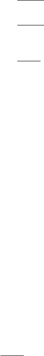
3.2.5 Canonical Decomposition
Any continuous linear system with constant coefficients can be transformed
into a special state-space form such that four separated subsystems result:
(A)controllable and observable subsystem,
(B)controllable and nonobservable subsystem,
(C)noncontrollable and observable subsystem,
(D)noncontrollable and nonobservable subsystem.
This division is called canonical decomposition and is shown in Fig. 3.8.
Only subsystem A can be calculated from input and output relations.
The system eigenvalues can be also divided into 4 groups:
(A)controllable and observable modes,
(B)controllable and nonobservable modes,
(C)noncontrollable and observable modes,
(D)noncontrollable and nonobservable modes.
State-space model of continuous linear systems with constant coefficients
is said to be minimal if it is controllable and observable.
State-space models of processes are more general than I/O models as they
can also contain noncontrollable and nonobservable parts that are cancelled
in I/O models.
Sometimes the notation detectability and stabilisability is used. A system
is said to be detectable if all nonobservable eigenvalues are asymptotically
stable and it is stabilisable if all nonstable eigenvalues are controllable.
84 3 Analysis of Process Models
(D)
(C)
(A)
(B)
-
-
-
u
y
Fig. 3.8. Canonical decomposition
3.3 Input-Output Process Models
In this section we focus our attention to transfer properties of processes. We
show the relations between state-space and I/O models.
3.3.1 SISO Continuous Systems with Constant Coefficients
Linear continuous SISO (single input, single output) systems with constant
coefficients with input u(t) and output y(t) can be described by a differential
equation in the form
a
n
d
n
y(t)
dt
n
+a
n−1
d
n−1
y(t)
dt
n−1
+···+a
0
y(t)=b
m
d
m
u(t)
dt
m
+···+b
0
u(t) (3.116)
where we suppose that u(t)andy(t) are deviation variables. After taking the
Laplace transform and assuming zero initial conditions we get
(a
n
s
n
+ a
n−1
s
n−1
+ ···+ a
0
)Y (s)=(b
m
s
m
+ ···+ b
0
)U(s) (3.117)
or
G(s)=
Y (s)
U(s)
=
B(s)
A(s)
(3.118)
where
B(s)=b
m
s
m
+ b
m−1
s
m−1
+ ···+ b
0
A(s)=a
n
s
n
+ a
n−1
s
n−1
+ ···+ a
0
3.3 Input-Output Process Models 85
G(s) is called a transfer function of the system and is defined as the ratio
between the Laplace transforms of output and input with zero initial condi-
tions.
Note 3.2. Transfer functions use the variable s of the Laplace transform. In-
troducing the derivation operator p =d/dt then the relation
G(p)=
Y (p)
U(p)
=
B(p)
A(p)
(3.119)
is only another way of writing Eq. (3.116).
A transfer function G(s) corresponds to physical reality if
n ≥ m (3.120)
Consider the case when this condition is not fulfilled, when n =1,m =0
a
0
y = b
1
du
dt
+ b
0
u (3.121)
If u(t)=1(t) (step change) then the system response is given as a sum of two
functions. The first function is an impulse function and the second is a step
function. As any real process cannot show on output impulse behaviour, the
case n<mdoes not occur in real systems and the relation (3.120) is called
the condition of physical realisability.
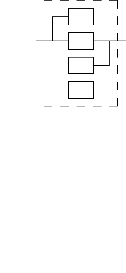
The relation
Y (s)=G(s)U(s) (3.122)
can be illustrated by the block scheme shown in Fig. 3.9 where the block
corresponds to G(s). The scheme shows that if input to system is U (s) then
output is the function G(s)U(s).
G(s)
- -
U(s) Y (s)
Fig. 3.9. Block scheme of a system with transfer function G(s)
Example 3.9: Transfer function of a liquid storage system
Consider the tank shown in Fig. 2.1. State-space equations for this system
are of the form (see 2.5)
dx
1
dt
= a
11
x
1
+ b
11
u
y
1
= x
1
where x
1
= h − h
s
,u = q
0
− q
s
0
. After taking the Laplace transform and
considering the fact that x
1
(0) = 0 follows
86 3 Analysis of Process Models
sX
1
(s)=a
11
X
1
(s)+b
11
U(s)
Y
1
(s)=X
1
(s)
and
(s −a
11
)Y
1
(s)=b
11
U(s)
Hence, the transfer function of this process is
G
1
(s)=
b
0
a
1
s +1
=
Z
1
T
1
s +1
where a
1
= T
1
=(2F
√
h
s
)/k
11
, b
0
= Z
1
=(2
√
h
s
)/k
11
. T
1
is time constant
and Z
1
gain of the first order system.
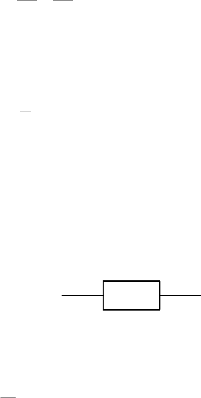
Example 3.10: Two tanks in a series - transfer function
Consider two tanks shown in Fig. 3.10. The level h
1
is not influenced by
the level h
2
.
q
0
h
q
1
h
1
2
q
2
F
1
F
2
Fig. 3.10. Two tanks in a series
The dynamical properties of the first tank can be described as
F
1
dh
1
dt
= q
0
− q
1
and the output equation is of the form
q
1
= k
11
h
1
The dynamical properties can also be written as
dh
1
dt
= f
1
(h
1
,q
0
)