Neubauer A., Freudenberger J., Kuhn V. Coding theory: algorithms, architectures and applications
Подождите немного. Документ загружается.

76 ALGEBRAIC CODING THEORY
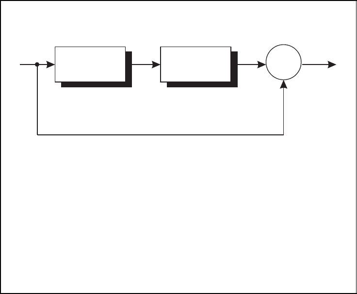
Syndrome decoding of a cyclic code
Syndrome
Calculation
Table
Lookup
+
-
+
r(z)
s(z)
ˆe(z)
ˆ
b(z)
■ The syndrome polynomial s(z) is calculated with the help of the received
polynomial r(z) and the generator polynomial g(z) according to
s(z) ≡ r(z) mod g(z) (2.70)
■ The syndrome polynomial s(z) is used to address a table that for each
syndrome stores the respective decoded error polynomial ˆe(z).
■ By subtracting the decoded error polynomial ˆe(z) from the received poly-
nomial r(z), the decoded code polynomial is obtained by
ˆ
b(z) = r(z) −ˆe(z) (2.71)
Figure 2.48: Syndrome decoding of a cyclic code with a linear feedback shift register
and a table look-up procedure. Reproduced by permission of J. Schlembach Fachverlag
Since g(z) divides the polynomial z
n
− 1, the generator polynomial of degree deg(g(z)) =
n − k can be defined by the corresponding set of zeros α
i
1
, α
i
2
, ..., α
i
n−k
. This yields
g(z) = (z − α
i
1
)(z− α
i
2
) ···(z − α
i
n−k
).
However, not all possible choices for the zeros are allowed because the generator poly-
nomial g(z) of a cyclic code B(n,k,d) over the finite field F
q
must be an element of
the polynomial ring F
q
[z], i.e. the polynomial coefficients must be elements of the finite
field F
q
. This is guaranteed if for each root α
i
its corresponding conjugate roots α
iq
, α
iq
2
,
... are also zeros of the generator polynomial g(z). The product over all respective linear
factors yields the minimal polynomial
m
i
(z) = (z − α
i
)(z− α
iq
)(z− α
iq
2
) ···

ALGEBRAIC CODING THEORY 77
Cyclotomic cosets and minimal polynomials
■ Factorisation of z
7
− 1 = z
7
+ 1 over the finite field F
2
into minimal polyno-
mials
z
7
+ 1 = (z + 1)(z
3
+ z + 1)(z
3
+ z
2
+ 1)
■ Cyclotomic cosets C
i
=
i 2
j
mod 7 : 0 ≤ j ≤ 2
C
0
={0}
C
1
={1, 2, 4}
C
3
={3, 6, 5}
Figure 2.49: Cyclotomic cosets and minimal polynomials over the finite field F
2
with coefficients in F
q
. The set of exponents i, iq, iq
2
, ... of the primitive nth root of
unity α ∈ F
q
l
corresponds to the so-called cyclotomic coset (Berlekamp, 1984; Bossert,
1999; Ling and Xing, 2004; McEliece, 1987)
C
i
=
iq
j
mod q
l
− 1:0≤ j ≤ l − 1
which can be used in the definition of the minimal polynomial
m
i
(z) =
κ∈C
i
(z − α
κ
).
Figure 2.49 illustrates the cyclotomic cosets and minimal polynomials over the finite field
F
2
. The generator polynomial g(z) can thus be written as the product of the corresponding
minimal polynomials. Since each minimal polynomial occurs only once, the generator
polynomial is given by the least common multiple
g(z) = lcm
m
i
1
(z), m
i
2
(z), . . . , m
i
n−k
(z)
.
The characteristics of the generator polynomial g(z) and the respective cyclic code
B(n,k,d) are determined by the minimal polynomials and the cyclotomic cosets respect-
ively.
A cyclic code B(n,k,d) with generator polynomial g(z) can now be defined by the set
of minimal polynomials or the corresponding roots α
1
, α
2
, ..., α
n−k
. Therefore, we will
denote the cyclic code by its zeros according to
B(n,k,d) = C(α
1
,α
2
,...,α
n−k
).

78 ALGEBRAIC CODING THEORY
Because of g(α
1
) = g(α
2
) =···=g(α
n−k
) = 0 and g(z) |b(z), the zeros of the generator
polynomial g(z) are also zeros
b(α
1
) = b(α
2
) =···=b(α
n−k
) = 0
of each code polynomial b(z) ∈ C(α
1
,α
2
,...,α
n−k
).
BCH Bound
Based on the zeros α
1
, α
2
, ..., α
n−k
of the generator polynomial g(z), a lower bound for
the minimum Hamming distance d of a cyclic code C(α
1
,α
2
,...,α
n−k
) has been derived
by Bose, Ray-Chaudhuri and Hocquenghem. This so-called BCH bound, which is given
in Figure 2.50, states that the minimum Hamming distance d is at least equal to δ if there
are δ − 1 successive zeros α
β
, α
β+1
, α
β+2
, ..., α
β+δ−2
(Berlekamp, 1984; Jungnickel,
1995; Lin and Costello, 2004).
Because of g(z) |b(z) for every code polynomial b(z), the condition in the BCH bound
also amounts to b(α
β
) = b(α
β+1
) = b(α
β+2
) =···=b(α
β+δ−2
) = 0. With the help of the
code polynomial b(z) = b
0
+ b
1
z + b
2
z
2
+···+b
n−1
z
n−1
, this yields
b
0
+ b
1
α
β
+ b
2
α
β 2
+ ···+b
n−1
α
β(n−1)
= 0,
b
0
+ b
1
α
β+1
+ b
2
α
(β+1) 2
+ ···+b
n−1
α
(β+1)(n−1)
= 0,
b
0
+ b
1
α
β+2
+ b
2
α
(β+2) 2
+ ···+b
n−1
α
(β+2)(n−1)
= 0,
.
.
.
b
0
+ b
1
α
β+δ−2
+ b
2
α
(β+δ−2) 2
+ ···+b
n−1
α
(β+δ−2)(n−1)
= 0
BCH bound
■ Let C(α
1
,α
2
,...,α
n−k
) be a cyclic code of code word length n over the
finite field F
q
with generator polynomial g(z),andletα ∈ F
q
l
be an nth root
of unity in the extension field F
q
l
with α
n
= 1.
■ If the cyclic code incorporates δ − 1 zeros
α
β
,α
β+1
,α
β+2
,...,α
β+δ−2
according to
g(α
β
) = g(α
β+1
) = g(α
β+2
) =···=g(α
β+δ−2
) = 0
the minimum Hamming distance d of the cyclic code is bounded below by
d ≥ δ (2.72)
Figure 2.50: BCH bound
ALGEBRAIC CODING THEORY 79
which corresponds to the system of equations
1 α
β
α
β 2
··· α
β(n−1)
1 α
β+1
α
(β+1) 2
··· α
(β+1)(n−1)
1 α
β+2
α
(β+2) 2
··· α
(β+2)(n−1)
.
.
.
.
.
.
.
.
.
.
.
.
.
.
.
1 α
β+δ−2
α
(β+δ−2) 2
··· α
(β+δ−2)(n−1)
b
0
b
1
b
2
.
.
.
b
n−1
=
0
0
0
.
.
.
0
.
By comparing this matrix equation with the parity-check equation Hb
T
= 0 of general
linear block codes, we observe that the (δ − 1) × n matrix in the above matrix equation
corresponds to a part of the parity-check matrix H. If this matrix has at least δ − 1 lin-
early independent columns, then the parity-check matrix H also has at least δ − 1 linearly
independent columns. Therefore, the smallest number of linearly dependent columns of H,
and thus the minimum Hamming distance, is not smaller than δ, i.e. d ≥ δ. If we consider
the determinant of the (δ − 1) × (δ − 1) matrix consisting of the first δ − 1 columns, we
obtain (Jungnickel, 1995)
1 α
β
α
β 2
··· α
β(δ−2)
1 α
β+1
α
(β+1) 2
··· α
(β+1)(δ−2)
1 α
β+2
α
(β+2) 2
··· α
(β+2)(δ−2)
.
.
.
.
.
.
.
.
.
.
.
.
.
.
.
1 α
β+δ−2
α
(β+δ−2) 2
··· α
(β+δ−2)(δ−2)
=
11 1 ··· 1
1 α
1
α
2
··· α
δ−2
1 α
2
α
4
··· α
2 (δ−2)
.
.
.
.
.
.
.
.
.
.
.
.
.
.
.
1 α
δ−2
α
(δ−2) 2
··· α
(δ−2)(δ−2)
α
β(δ−1)(δ−2)/2
.
The resulting determinant on the right-hand side corresponds to a so-called Vander-
monde matrix, the determinant of which is different from 0. Taking into account that
α
β(δ−1)(δ−2)/2
= 0, the (δ − 1) × (δ − 1) matrix consisting of the first δ − 1 columns is
regular with δ − 1 linearly independent columns. This directly leads to the BCH bound
d ≥ δ.
According to the BCH bound, the minimum Hamming distance of a cyclic code is
determined by the properties of a subset of the zeros of the respective generator polynomial.
In order to define a cyclic code by prescribing a suitable set of zeros, we will therefore
merely note this specific subset. A cyclic binary Hamming code, for example, is determined
by a single zero α; the remaining conjugate roots α
2
, α
4
, ... follow from the condition
that the coefficients of the generator polynomial are elements of the finite field F
2
. The
respective cyclic code will therefore be denoted by C(α).
Definition of BCH Codes
In view of the BCH bound in Figure 2.50, a cyclic code with a guaranteed minimum
Hamming distance d can be defined by prescribing δ − 1 successive powers
α
β
,α
β+1
,α
β+2
,...,α
β+δ−2

80 ALGEBRAIC CODING THEORY
BCH codes
■ Let α ∈ F
q
l
be an nth root of unity in the extension field F
q
l
with α
n
= 1.
■ The cyclic code C(α
β
,α
β+1
,α
β+2
,...,α
β+δ−2
) over the finite field F
q
is
called the BCH code to the design distance δ.
■ The minimum Hamming distance is bounded below by
d ≥ δ (2.73)
■ A narrow-sense BCH code is obtained for β = 1.
■ If n = q
l
− 1, the BCH code is called primitive.
Figure 2.51: Definition of BCH codes
of an appropriate nth root of unity α as zeros of the generator polynomial g(z). Because
of
d ≥ δ
the parameter δ is called the design distance of the cyclic code. The resulting cyclic code
over the finite field F
q
is the so-called BCH code C(α
β
,α
β+1
,α
β+2
,...,α
β+δ−2
) to the
design distance δ (see Figure 2.51) (Berlekamp, 1984; Lin and Costello, 2004; Ling and
Xing, 2004). If we choose β = 1, we obtain the narrow-sense BCH code to the design
distance δ. For the code word length
n = q
l
− 1
the primitive nth root of unity α is a primitive element in the extension field F
q
l
due
to α
n
= α
q
l
−1
= 1. The corresponding BCH code is called a primitive BCH code. BCH
codes are often used in practical applications because they are easily designed for a wanted
minimum Hamming distance d (Benedetto and Biglieri, 1999; Proakis, 2001). Furthermore,
efficient algebraic decoding schemes exist, as we will see in Section 2.3.8.
As an example, we consider the cyclic binary Hamming code over the finite field F
2
with
n = 2
m
− 1 and k = 2
m
− m − 1. Let α be a primitive nth root of unity in the extension
field F
2
m
. With the conjugate roots α, α
2
, α
2
2
, ..., α
2
m−1
, the cyclic code
C(α) =
b(z) ∈ F
2
[z]/(z
n
− 1) : b(α) = 0
is defined by the generator polynomial
g(z) = (z − α) (z − α
2
)(z− α
2
2
) ···(z − α
2
m−1
).
ALGEBRAIC CODING THEORY 81
Owing to the roots α and α
2
there exist δ − 1 = 2 successive roots. According to the BCH
bound, the minimum Hamming distance is bounded below by d ≥ δ = 3. In fact, as we
already know, Hamming codes have a minimum Hamming distance d = 3.
In general, for the definition of a cyclic BCH code we prescribe δ − 1 successive zeros
α
β
, α
β+1
, α
β+2
, ..., α
β+δ−2
. By adding the corresponding conjugate roots, we obtain the
generator polynomial g(z) which can be written as
g(z) = lcm
m
β
(z), m
β+1
(z), . . . , m
β+δ−2
(z)
.
The generator polynomial g(z) is equal to the least common multiple of the respective
polynomials m
i
(z) which denote the minimal polynomials for α
i
with β ≤ i ≤ β + δ − 2.
2.3.7 Reed–Solomon Codes
As an important special case of primitive BCH codes we now consider BCH codes over
the finite field F
q
with code word length
n = q − 1.
These codes are called Reed–Solomon codes (Berlekamp, 1984; Bossert, 1999; Lin and
Costello, 2004; Ling and Xing, 2004); they are used in a wide range of applications ranging
from communication systems to the encoding of audio data in a compact disc (Costello
et al., 1998). Because of α
n
= α
q−1
= 1, the nth root of unity α is an element of the finite
field F
q
. Since the corresponding minimal polynomial of α
i
over the finite field F
q
is
simply given by
m
i
(z) = z − α
i
the generator polynomial g(z) of such a primitive BCH code to the design distance δ is
g(z) = (z − α
β
)(z− α
β+1
) ···(z − α
β+δ−2
).
The degree of the generator polynomial is equal to
deg(g(z)) = n − k = δ − 1.
Because of the BCH bound, the minimum Hamming distance is bounded below by d ≥ δ =
n − k + 1 whereas the Singleton bound delivers the upper bound d ≤ n − k + 1. Therefore,
the minimum Hamming distance of a Reed–Solomon code is given by
d = n − k + 1 = q − k.
Since the Singleton bound is fulfilled with equality, a Reed–Solomon code is an MDS
(maximum distance separable) code. In general, a Reed–Solomon code over the finite field
F
q
is characterised by the following code parameters
n = q − 1,
k = q −δ,
d = δ.
In Figure 2.52 the characteristics of a Reed–Solomon code are summarised. For practically
relevant code word lengths n, the cardinality q of the finite field F
q
is large. In practical
applications q = 2
l
is usually chosen. The respective elements of the finite field F
2
l
are
then represented as l-dimensional binary vectors over F
2
.

82 ALGEBRAIC CODING THEORY
Reed–Solomon codes
■ Let α be a primitive element of the finite field F
q
with n = q −1.
■ The Reed–Solomon code is defined as the primitive BCH code to the
design distance δ over the finite field F
q
with generator polynomial
g(z) = (z − α
β
)(z− α
β+1
) ···(z − α
β+δ−2
) (2.74)
■ Code parameters
n = q − 1 (2.75)
k = q −δ (2.76)
d = δ (2.77)
■ Because a Reed–Solomon code fulfils the Singleton bound with equality,
it is an MDS code.
Figure 2.52: Reed–Solomon codes over the finite field F
q
Spectral Encoding
We now turn to an interesting relationship between Reed–Solomon codes and the discrete
Fourier transform (DFT) over the finite field F
q
(Bossert, 1999; Lin and Costello, 2004;
Neubauer, 2006b) (see also Section A.4 in Appendix A). This relationship leads to an effi-
cient encoding algorithm based on FFT (fast Fourier transform) algorithms. The respective
encoding algorithm is called spectral encoding.
To this end, let α ∈ F
q
be a primitive nth root of unity in the finite field F
q
with
n = q − 1. Starting from the code polynomial
b(z) = b
0
+ b
1
z +···+b
n−2
z
n−2
+ b
n−1
z
n−1
the discrete Fourier transform of length n over the finite field F
q
is defined by
B
j
= b(α
j
) =
n−1
i=0
b
i
α
ij
•−◦ b
i
= n
−1
B(α
−i
) = n
−1
n−1
j=0
B
j
α
−ij
with b
i
∈ F
q
and B
j
∈ F
q
. The spectral polynomial is given by
B(z) = B
0
+ B
1
z +···+B
n−2
z
n−2
+ B
n−1
z
n−1
.
Since every code polynomial b(z) is divided by the generator polynomial
g(z) = (z − α
β
)(z− α
β+1
) ···(z − α
β+δ−2
)
ALGEBRAIC CODING THEORY 83
which is characterised by the zeros α
β
, α
β+1
, ..., α
β+δ−2
, every code polynomial b(z)
also has zeros at α
β
, α
β+1
, ..., α
β+δ−2
, i.e.
b(α
β
) = b(α
β+1
) = b(α
β+2
) =···=b(α
β+δ−2
) = 0.
In view of the discrete Fourier transform and the spectral polynomial B(z) •−◦ b(z), this
can be written as
B
j
= b(α
j
) = 0
for β ≤ j ≤ β +δ − 2. These spectral coefficients are called parity frequencies.
If we choose β = q − δ, we obtain the Reed–Solomon code of length n = q − 1,
dimension k = q − δ and minimum Hamming distance d = δ. The information polynomial
u(z) = u
0
+ u
1
z + u
2
z
2
+···+u
q−δ−1
z
q−δ−1
with k = q − δ information symbols u
j
is now used to define the spectral polynomial B(z)
according to
B(z) = u(z),
i.e. B
j
= u
j
for 0 ≤ j ≤ k − 1 and B
j
= 0 for k ≤ j ≤ n − 1. This setting yields B
j
=
b(α
j
) = 0 for q − δ ≤ j ≤ q − 2. The corresponding code polynomial b(z) is obtained
from the inverse discrete Fourier transform according to
b
i
=−B(α
−i
) =−
q−2
j=0
B
j
α
−ij
.
Here, we have used the fact that n = q − 1 ≡−1 modulo p, where p denotes the char-
acteristic of the finite field F
q
, i.e. q = p
l
with the prime number p. Finally, the spectral
encoding rule reads
b
i
=−
q−δ−1
j=0
u
j
α
−ij
.
Because there are fast algorithms available for the calculation of the discrete Fourier trans-
form, this encoding algorithm can be carried out efficiently. It has to be noted, however,
that the resulting encoding scheme is not systematic. The spectral encoding algorithm
of a Reed–Solomon code is summarised in Figure 2.53 (Neubauer, 2006b). A respective
decoding algorithm is given elsewhere (Lin and Costello, 2004).
Reed–Solomon codes are used in a wide range of applications, e.g. in communication
systems, deep-space applications, digital video broadcasting (DVB) or consumer systems
(Costello et al., 1998). In the DVB system, for example, a shortened Reed–Solomon code
with n = 204, k = 188 and t = 8 is used which is derived from a Reed–Solomon code over
the finite field F
2
8
= F
256
(ETSI, 2006). A further important example is the encoding of the
audio data in the compact disc with the help of the cross-interleaved Reed–Solomon code
(CIRC) which is briefly summarised in Figure 2.54 (Costello et al., 1998; Hoeve et al.,
1982).
84 ALGEBRAIC CODING THEORY
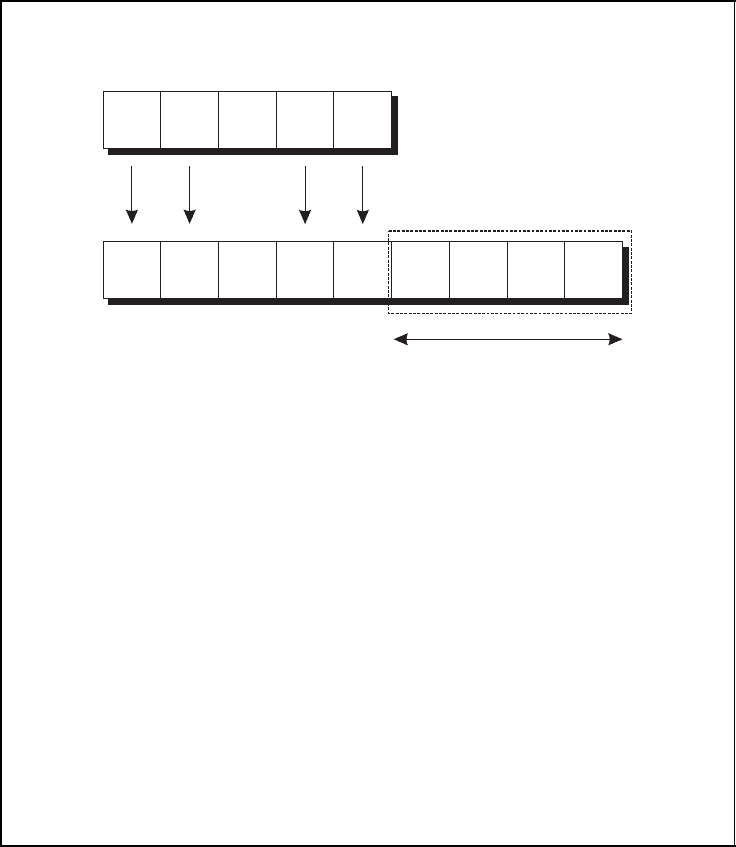
Spectral encoding of a Reed–Solomon code
...
......
...
u
0
u
1
u
k−2
u
k−1
B
0
B
1
B
k−2
B
k−1
000
δ − 1
■ The k information symbols are chosen as the first k spectral coefficients,
i.e.
B
j
= u
j
(2.78)
for 0 ≤ j ≤ k − 1.
■ The remaining n − k spectral coefficients are set to 0 according to
B
j
= 0 (2.79)
for k ≤ j ≤ n − 1.
■ The code symbols are calculated with the help of the inverse discrete
Fourier transform according to
b
i
=−B(α
−i
) =−
q−2
j=0
B
j
α
−ij
=−
q−δ−1
j=0
u
j
α
−ij
(2.80)
for 0 ≤ i ≤ n − 1.
Figure 2.53: Spectral encoding of a Reed–Solomon code over the finite field F
q
.
Reproduced by permission of J. Schlembach Fachverlag
2.3.8 Algebraic Decoding Algorithm
Having defined BCH codes and Reed–Solomon codes, we now discuss an algebraic
decoding algorithm that can be used for decoding a received polynomial r(z) (Berlekamp,
1984; Bossert, 1999; Jungnickel, 1995; Lin and Costello, 2004; Neubauer, 2006b). To
this end, without loss of generality we restrict the derivation to narrow-sense BCH codes

ALGEBRAIC CODING THEORY 85
Reed–Solomon codes and the compact disc
■ In the compact disc the encoding of the audio data is done with the help
of two interleaved Reed–Solomon codes.
■ The Reed–Solomon code with minimum distance d = δ = 5 over the finite
field F
256
= F
2
8
with length n = q − 1 = 255 and k = q − δ = 251 is short-
ened such that two linear codes B(28, 24, 5) and B(32, 28, 5) over the finite
field F
2
8
arise.
■ The resulting interleaved coding scheme is called CIRC (cross-interleaved
Reed–Solomon code).
■ For each stereo channel, the audio signal is sampled with 16-bit resolution
and a sampling frequency of 44.1 kHz, leading to a total of 2 × 16 ×44 100 =
1 411 200 bits per second. Each 16-bit stereo sample represents two 8-bit
symbols in the field F
2
8
.
■ The inner shortened Reed–Solomon code B(28, 24, 5) encodes 24 infor-
mation symbols according to six stereo sample pairs.
■ The outer shortened Reed–Solomon code B(32, 28, 5) encodes the resul-
ting 28 symbols, leading to 32 code symbols.
■ In total, the CIRC leads to 4 231 800 channel bits on a compact disc which
are further modulated and represented as so-called pits on the compact
disc carrier.
Figure 2.54: Reed–Solomon codes and the compact disc
C(α, α
2
,...,α
δ−1
) with α ∈ F
q
l
of a given designed distance
δ = 2t + 1.
It is important to note that the algebraic decoding algorithm we are going to derive is only
capable of correcting up to t errors even if the true minimum Hamming distance d is larger
than the designed distance δ. For the derivation of the algebraic decoding algorithm we
make use of the fact that the generator polynomial g(z) has as zeros δ − 1 = 2t successive
powers of a primitive nth root of unity α, i.e.
g(α) = g(α
2
) =···=g(α
2t
) = 0.
Since each code polynomial
b(z) = b
0
+ b
1
z +···+b
n−2
z
n−2
+ b
n−1
z
n−1