Odekon M. Encyclopedia of paleoclimatology and ancient environments

Подождите немного. Документ загружается.

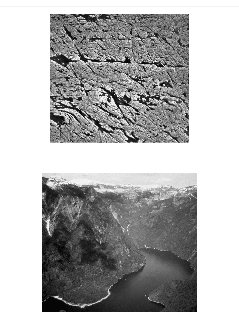
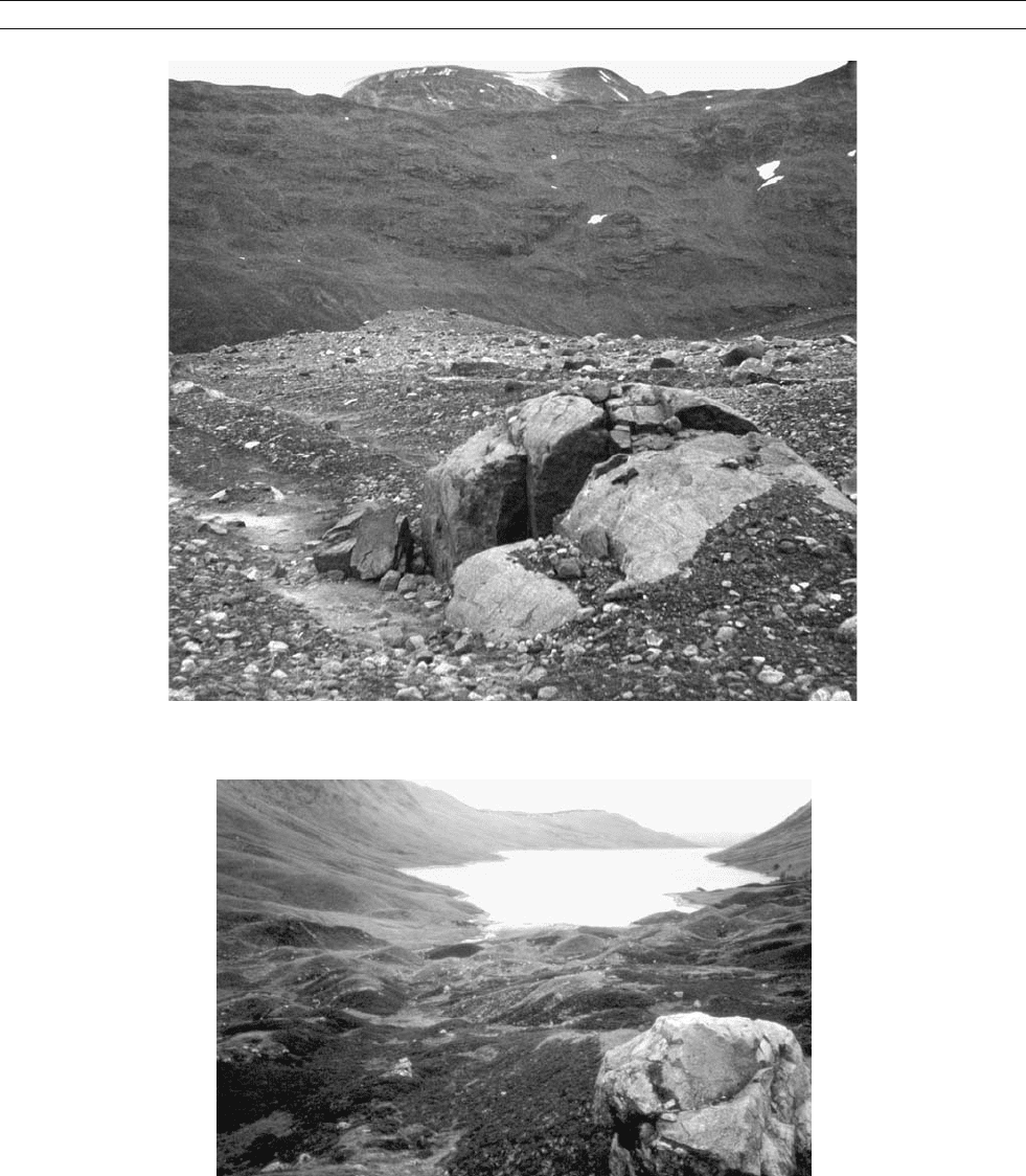
Figure G26 Areally scoured glaciated terrain near Lac Troie, Quebec, Canada.

Figure G27 Princess Louise Inlet, British Columbia, Canada.

GLACIAL GEOMORPHOLOGY 367

bedrock knob landscapes, such as the Canadian and Fennos-

candian Shields, for example Bennett & Glasser, 1996; Benn

& Evans, 1998.

Glacial transport

Glaciers and ice sheets transport vast quantities of sediment

from fine-grained clays and silts to huge boulders. Sediment is

transported on the surface of the ice as supraglacial debris,

within the ice as englacial debris, beneath the ice as subglacial

debris, and beyond the ice margins as proglacial sediment.

Each environment affixes the transported sediment with a

potentially distinctive signature that, although complex due

to overprinting and re-transportation, can be used, at times, to

differentiate glacial sediment types Bennett & Glasser, 1996;

Benn & Evans, 1998; Menzies, 2002. Sediment is transpor-

ted encased within the basal layers of the ice, on the surface

of the ice, and beneath the ice within deforming soft sedi-

ment beds.

Glacial deposition: processes, landforms, and

landscape systems

The deposition of glacial sediment is largely a function of the

means of sediment transportation. Since ice masses scavenge

sediments from their glaciated basins, and in the case of ice sheets

this may be continental landmasses, the provenance of glacial

sediment is typically immense, containing far-traveled sediment

and boulders as well as local rock materials. In fact, most glacial

sediments reflect a provenance only a few 10s of kilometers up-

ice from any point of deposition. However, repeated glaciation

may greatly increase the original distance from the origin to the

final deposition site.

Glacial deposits occur as unsorted sediments with a wide range

of particle sizes and as sorted sediments deposited by meltwater.

Unsorted sediments are typically referred to as till or glacial

diamicton. These sediments are exceedingly complex sedimento-

logically and stratigraphically. They occur in all sub-environments

of the glacier system and range from subglacial clay-rich,

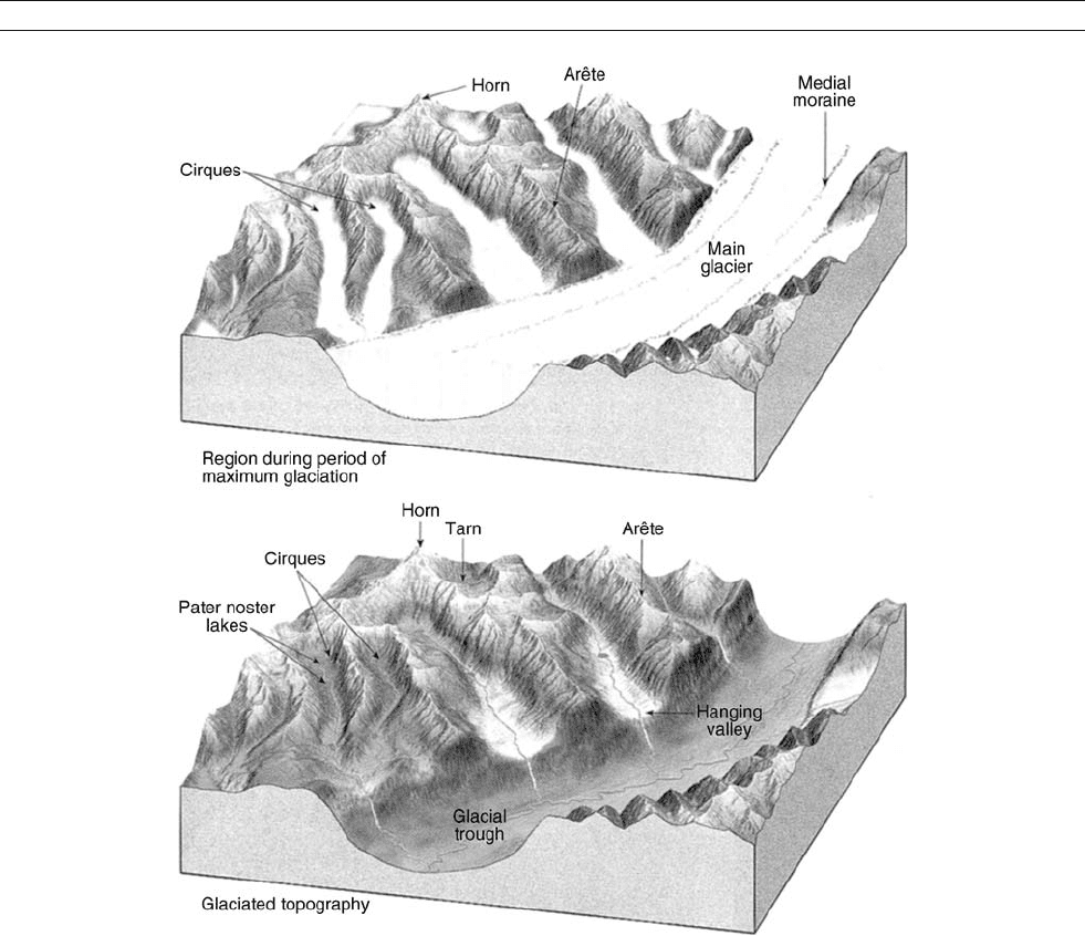
Figure G28 Erosional landscape system for alpine glaciation (modified from Tarbuck and Lutgens, 2003).

368 GLACIAL GEOMORPHOLOGY

consolidated lodgement tills to coarse supraglacial flow tills,

and subglacial and submarginal areas of basal ice melting leading

to melt-out tills. However, this classification with reference to

subglacial tills is probably inaccurate. It would be more rigorous

to term these tills “tectomicts,” products of the complex subglacial

environment.

The sorted or fluvioglacial sediments range from fine-

grained clays deposited in glacial lakes (glaciolacustrine) to

coarser sands and gravels deposited in front of ice masses as

outwash fans or sandur, and rain-out sediments deposited in

marine settings (glaciomarine).

Processes

The processes of glacial deposition range from direct smearing

of subglacial debris as lodgement tills to mass movement of

sediments from the frontal and lateral margins of glaciers as flow

tills, and to direct ablation of ice forming melt-out tills in front

of ice masses in proglacial areas and within subglacial cavities.

Landforms

Glacial landforms include those formed (a) transverse to ice

motion, (b) parallel to ice motion, (c) unoriented, non-linear,

(d) ice marginal, and (e) fluvioglacial. Although a complex

myriad of glacial depositionary forms occur in most glaciated

areas, the dominant landforms discussed below include

(a) Rogen moraines, (b) drumlins and fluted moraines, (c) hum-

mocky moraines, (d) end moraines, and (e) eskers and kames.

Rogen moraines or ribbed moraines are a series of conspic-

uous ridges formed transverse to ice movement. These ridges

typically rise 10–20 m in height, 50–100 m in width, and are

spaced 100–300 m apart. They tend to occur in large numbers

as fields, for example, in the Mistassini area of Quebec. They

are composed of a range of subglacial sediments and are

thought to be formed by the basal deformation of underlying

sediment, possibly in association with a floating ice margin at

times ( Figure G29 ) Menzies, 2002.

Drumlins are perhaps one of the most well known glacial

landforms. Considerable literature exists on their formation

and debate continues on their mechanic(s) of formation. Drum-

lins are streamlined, roughly elliptical or ovoid-shaped hills

with a steep stoss side facing up-ice and a gentler lee-side

facing down-ice (Figure G30a). Drumlins range in height from

a few meters to over 250 m, and may be from 100 m to several

kilometers in length (Figure G30b). They tend to be found in

vast swarms or fields of many thousands (Figure G30b). In

central New York State, for example, over 70,000 occur, and

vast fields likewise exist in Finland, Poland, Scotland, and

Canada. Drumlins are composed of a wide range of subglacial

sediments and may contain boulder cores, bedrock cores, sand

dikes, and “rafted” non-glacial sediments. It seems likely that

these landforms develop below relatively fast moving ice

beneath which a deforming layer of sediment develops inequal-

ities and preferentially stiffer units become nuclei around which

sediment accumulates and the characteristic shape evolves.

Other hypotheses of formation range from the streamlining

of pre-existing glacial sediments by erosion, to changes in the

dilatancy of glacial sediments leading to stiffer nuclei at the

ice-bed interface, fluctuations in porewater content and pressure

within subglacial sediments again at the ice-bed interface, and

the infilling of subglacial cavities by massive subglacial floods.

Fluted moraines are regarded as subglacial streamlined

bedforms akin to drumlins (Figure G31). These landforms are

typically linked in formation with drumlins and Rogen mor-

aines. They tend to be much smaller in height and width than

drumlins but may stretch for tens of kilometers in length. They

are typically composed of subglacial sediments. Fluted mor-

aines have been found to develop in the lee of large boulders

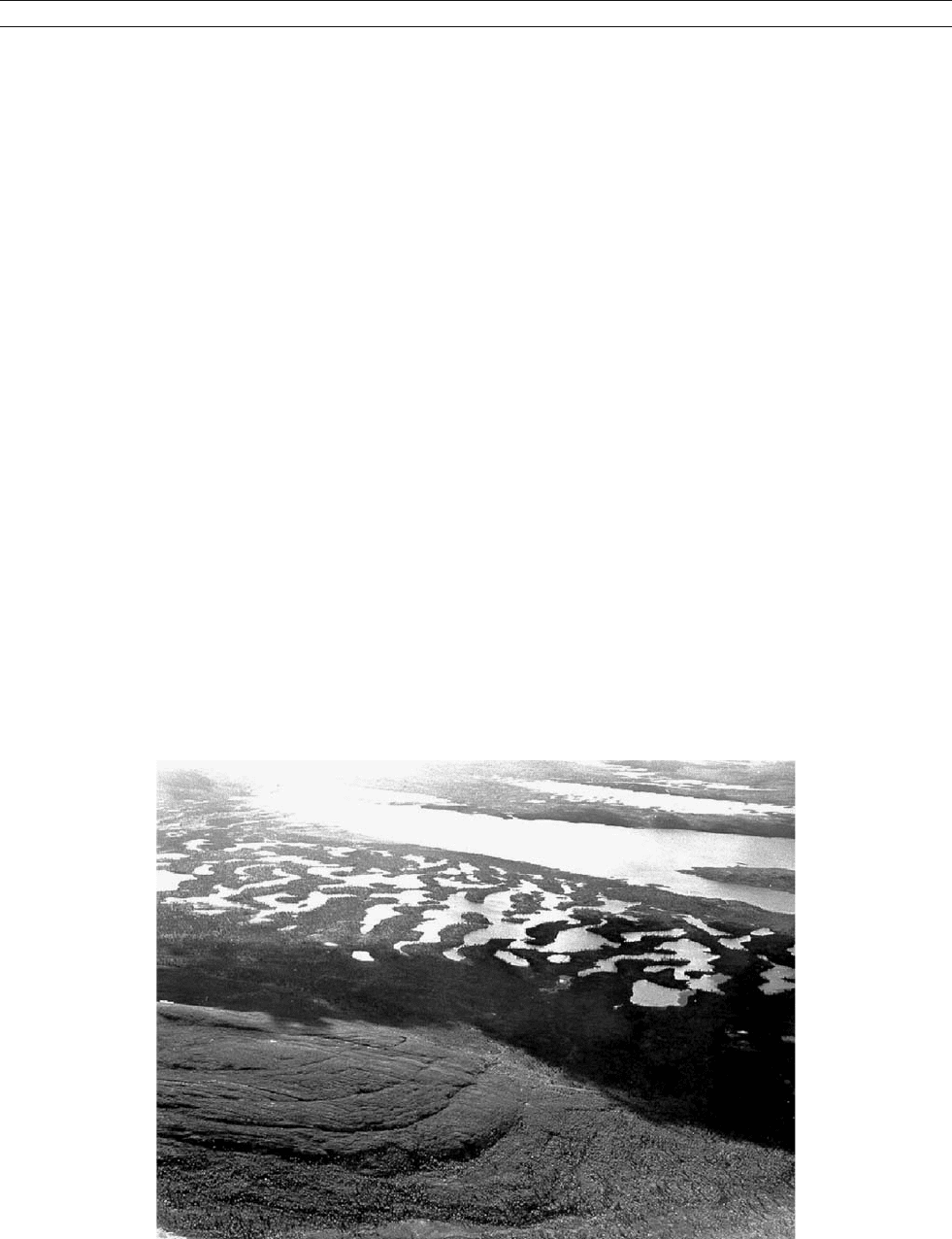
Figure G29 Rogen moraine near Uthusslo

n, Sweden (photo from Jan Lunqvist).

GLACIAL GEOMORPHOLOGY 369

but may also be attenuated drumlin forms, the result of high

basal ice shear stress and high ice velocities. In central New

York State, fluted moraines occur beside and amongst the large

drumlin fields.

Hummocky moraine is a term used to denote an area of ter-

rain in which a somewhat chaotic deposition pattern occurs,

similar to a series of small sediment dumps (Figure G32). These

moraines rarely rise above a few meters but may extend over

considerable areas. Hummocky moraines often mark locations

where massive down-wasting of an ice mass may have occurred.

End or terminal moraines and retreat or frontal moraines

occur at the front margins of ice masses. Typically, these land-

forms, transverse to ice motion, are a few meters to tens of

meters in height and, if built-up over several years, may be

even higher and of some considerable width (1–5 km). Mor-

aines contain subglacial and supraglacial debris, and often have

an acurate shape closely mirroring the shape of an ice front.

Since these moraines mark the edge of an ice mass at any given

time, the longer ice remains at that location, the higher and

larger the moraines become. However, as an ice mass retreats,

with periodic stationary periods (stillstands), a series or sequence

of moraines (i.e., recessional moraines) develop that mark the

retreatstagesoftheice(Figure G33). Sequences of end moraines

can be observed in the mid-west states of Illinois, Ohio, and

Michigan Mickelson & Attig, 1999.

Eskers are products of subglacial meltwater streams in

which the meltwater channel has become blocked by fluviogla-

cial sediments. Eskers are long ridges of sands and gravels that

form anatomizing patterns across the landscape (Figure G34).

They range in height from a few meters to > 50 m and may

run for tens of kilometers. In Canada, some eskers cross the

Canadian Shield for hundreds of kilometers. These landforms

often have branching ridges and a dendritic morphology.

Eskers are dominantly composed of fluvioglacial sands and

gravels with distinctive faulted strata along the edges where

the ice tunnel wall melted and collapsed. In many instances

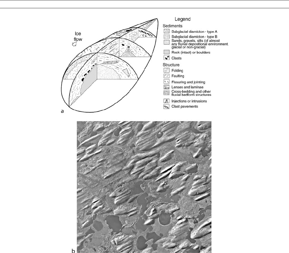
Figure G30 (a) General model of drumlin plan and variability of internal composition, (b) drumlin field in Saskatchewan (ice direction from

upper right to lower left).

370 GLACIAL GEOMORPHOLOGY

eskers are observed “running” uphill or obliquely crossing over

drumlins, a testament to their formation within high pressure

subglacial meltwater tunnels Benn & Evans, 1998.

In many glaciated areas during ice retreat, large, roughly cir-

cular dumps of fluvioglacial sands and gravels occur. These

forms, termed kames, appear to form when infilled crevasses

or buried ice melt, leaving the sediment behind in a complex

but chaotic series of mounds. The term kame or kame-delta

has been applied to fluvioglacial sediments that have formed

temporary deltas into long-gone glacial lakes. In Finland, a

long line of such kame-deltas formed into a moraine-like series

of linear ridges transverse to ice front retreat (Salpuasselkä).

Figure G31 Fluted moraine, Storbreen Glacier, Norway (boulder at the head of the flute; ice direction bottom right to middle left).

Figure G32 Hummocky moraine, Glen Turret, Scotland.

GLACIAL GEOMORPHOLOGY 371

Glacial depositional landscape systems

Distinctive suites of glacial depositional landforms can be

found in valley glacier, and ice sheet settings (Figure G35).

Typically, these sequences of landforms are often overprinted

due to subsequent glaciations but in the mid-west of the

USA, such suites of depositional landforms from the last gla-

ciation to affect the area (Late Wisconsinan) can be clearly dis-

cerned (Figure G33). Distinctive landscape systems attributable

to the marginal areas of ice sheets also carry a unique supragla-

cial suite of landforms, as can be observed in parts of the mid-

western USA (Figure G36 ).

The impact o f glaciation beyond ice limits

Areas beyond the ice limits are greatly influenced by glaciation

due to deteriorating climatic conditions, the deposition of wind-

blown dust (loess), the divergence of river systems where head-

waters or partial drainage basins may be intersected by advancing

ice, the impact of outburst floods from ice fronts (jökulhlaups),

and major faunal and floral changes due to encroaching ice. In

terms of the impact of ice masses on human life and society,

the only evidence is somewhat anecdotal. At the close of the Late

Wisconsinan, ice masses may have acted to spur human migration,

for example through the short-lived ice-free corridor between the

Cordilleran and Laurentian Ice Sheets in central Alberta, Canada

into the prairies to the south.

Within a few hundreds of kilometers of the vast ice sheets

that covered North America and Europe, significant climatic

conditions must have been severe with strong katabatic cold

winds descending from the ice. Associated with these severe

climates, periglacial conditions must have prevailed, in which

the ground became permanently frozen to a considerable depth.

The effects of periglacial activity produced frozen ground phe-

nomena such as solifluction sediments down slopes, ice and

sand wedges, and localized ice lenses and pingo formation.

Dramatic changes in vegetation types and animal life occurred,

with the southern migration of many species in the Northern

Hemisphere. For example, unlike today, central southern Texas

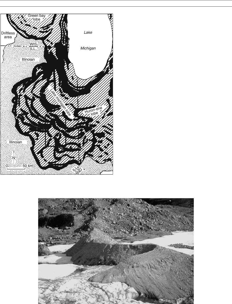
Figure G33 Late Wisconsinan end moraines (black) of the Green Bay

Lobe (Wisconsin), Lake Michigan Lobe, and Huron-Erie Lobe (Indiana)

(modified after Frye and Willman, 1973).

Figure G34 Esker Ridge, Bylot Island, Canada (photograph courtesy of C. Zdanowicz).

372 GLACIAL GEOMORPHOLOGY

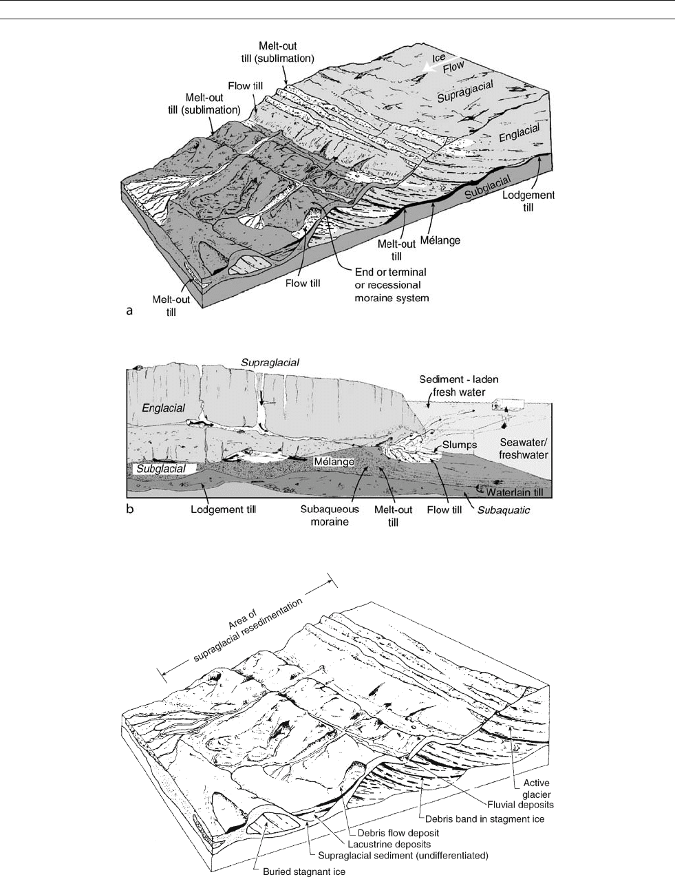
Figure G35 (a) Model of land-based glacial depositional system. (b) Model of depositional system of an ice mass with a marine margin.

Figure G36 (a) Model of supraglacial and ice-marginal landscape systems (modified from Edwards, 1986). (b) Supraglacial and ice-marginal

landscapes, Findeln Glacier, Switzerland.

GLACIAL GEOMORPHOLOGY 373

would have supported hardwood forests of the type now found

in Ohio and Pennsylvania.

Due to the katabatic winds, fine sediments were picked up

from the proglacial areas along the margins of the ice sheets

and the dust was transported away from the ice and deposited

as thick, massive loess sediments (glacioaeolian sediments).

Considerable thicknesses of these sediments occur in the mid-

western states of the USA, especially in Iowa and Kansas,

and also in central Europe, Hungary, Central Asia, and China.

In some instances, vast outpourings of meltwater (jökulhlaups)

flooded from the ice fronts, leading to distinctive, heavily dis-

sected terrains being formed (badlands). Such an occurrence

is recorded in the Columbia River Badlands of Washington and

Oregon States where a huge lake formed and then dramatically

drained (Lake Missoula floods) (Figure G37).

John Menzies

Bibliography

Benn, D.I., and Evans, D.J.A., 1998. Glaciers and Glaciation. London:

Arnold Publishers, 734pp.

Bennett, M.R., and Glasser, N.F., 1996. Glacial Geology. Chichester: Wiley

publishers.

Menzies, J. (ed.), 2002. Modern and Past Glacial Environments (Student

Edition). Oxford: Butterworth-Heineman, 543pp.

Mickelson, D., and Attig, J. (eds.), 1999. Glacial Processes Past and Present.

Special paper 337, Boulder, CO: Geological Society of America.

Cross-references

Cirques

Cryosphere

Diamicton

Drumlins

Eskers

Glacial Erratics

Glacial Megalakes

Glaciations, Quaternary

Glaciations, Pre-Quaternary

Glaciofluvial Sediments

Icehouse (cold) Climates

Kames

Kettles

Late Quaternary Megafloods

Loess Deposits

Moraines

Mountain Glaciers

Periglacial Geomorphology

Pingos

Roche Moutonnées

GLACIAL ISOSTASY

Glacial isostasy refers to the response of the solid Earth to any

changes in the planet’s ice sheets. The Earth is not a rigid body

and it will deform when subjected to forces or to changes in sur-

face loads. The nature of this deformation depends largely on the

time scale, magnitude, and wavelength of the deforming force or

load. Examples include the very rapid crustal fracturing at the

time of earthquakes, the semi-diurnal and diurnal tidal deforma-

tions of the solid planet due to the changing gravitational attrac-

tion by the Sun and Moon, and the seasonal changes in the mass

distribution within the atmosphere. Examples on longer, geologi-

cal timescales include the redistribution of surface loads during

erosion and sediment deposition or by the formation of large vol-

canic complexes. At the high frequency part of the spectrum, the

response is primarily elastic but with decreasing frequency the

response becomes increasingly viscous.

To a first approximation, the Earth is a layered body whose

outer shell, the lithosphere, acts essentially as an elastic layer.

The mantle below is more viscous and flows when subject to

non-hydrostatic stress and for very long term loads, of the order

of a million years or more, this region behaves largely as a

fluid. The outer core acts as a fluid even at high frequencies.

The lithosphere comprises the crust, which is relatively cold

and brittle, and the uppermost part of the mantle that is rela-

tively cool, strong, and elastic.

Isostasy is a concept that describes the response of the pla-

net to a change in surface load. It was originally developed to

describe the mechanism by which mountains and plateaus were

supported by the crust for long periods of time. In its simplest

Figure G37 Jo

kulhlaup resulting from catastrophic drainage of glacial Lake Missoula has led to the formation of the Channeled Scablands of

Washington and Oregon.

374 GLACIAL ISOSTASY

form, the surface load is assumed to be underlain by lower-

than-normal densities such that below the crust or lithosphere

the pressures are hydrostatic everywhere. The manner in which

this “compensating” mass is distributed gives rise to different

models of isostasy: Airy, Pratt, or regional. The first two models

are local compensation models in which the compensating mass

is located immediately below the load but in the third model, a

local load is supported regionally. The underlying assumption

in these models is that the surface loads are supported by stresses

within the crust-lithosphere and that the sub-lithospheric mantle

is fluid, an assumption that is operationally effective on long

timescales of many tectonic processes.

Glacial isostasy is concerned with the planet’s response to

the changing surface loads of ice and water during the waxing

and waning of large ice sheets. To a first approximation of local

isostasy, the crust beneath the ice sheet is depressed by the pro-

duct of the ratio of ice and mantle densities and the thickness of

the ice, such that somewhere below the ice-loaded lithosphere

the vertical pressures are constant at constant depth. For a

3 km thick ice cap, this would mean a crustal depression of

about 800 m. On timescales of glacial cycles (10

–10

years),

the mantle does not behave as a fluid and the load will be partly

supported by viscous stresses in the sub-lithospheric region.

Thus, the initial response to a large ice load will be by elastic

deformation of the entire lithosphere-mantle followed by a

viscous creep as the mantle stresses relax and the load is

increasingly supported by the lithosphere. The local isostatic

depression will be attained as a limit. Likewise, when the ice

sheet is removed, the initial response is elastic followed by a

viscous rebound. The rate at which this occurs will be a func-

tion of the mantle viscosity and observations of this rebound,

in fact, provide the primary evidence for this viscosity.

Large ice sheets have periodically formed on the Earth’s

surface in response to changes in planetary configurations and

the resulting changes in solar insolation (e.g., the Milankovitch

theory). Thus, water mass is withdrawn from the oceans and

localized at high latitudes when large ice sheets form, and more

than 50  10

of water is periodically moved between the

ice sheets and the oceans, resulting in a global lowering of sea

level by 130–150 m. This is the most direct consequence of

glacial isostasy: global fluctuations in sea level that mirror the

growth and decay of ice sheets during the glacial cycles of

the past two million years. The spatial pattern of this sea-level

change is, however, complex. What is observed is that the posi-

tion of past shorelines relative to the present shoreline position

and the crust – which forms the reference surface for the mea-

surement – is itself displaced during the surface-loading cycles.

Moreover, as the Earth deforms and mass is redistributed

around the globe, the gravity field of the planet changes and

surfaces of constant gravitational potential, e.g., the geoid or

sea level in the absence of oceanographic and meteorological

forcing, are modified as well. Thus, the relative sea-level obser-

vation at a locality is a measure of the change in ocean volume,

of the radial deformation of the Earth’s surface under the chan-

ging surface load, and of the change in gravitational potential.

The globally averaged sea-level change resulting from a change

in ice volume is referred to as the ice-volume-equivalent sea-

level change and, in the absence of other processes that change

ocean volume, this corresponds to eustatic sea-level change.

The Earth is presently in an interglacial period and the last

of the large ice sheets over North America and Europe disap-

peared before ~7,000 years ago. The remaining ice sheets

of Greenland and Antarctica also, in a first approximation,

stabilized by about this time. However, while ocean volumes

remained nearly constant during the interglacial period, sea

levels have continued to change as a result of the viscous or

delayed response of the Earth to the removal of the ice load

and the redistribution of the melt water into the oceans. The

amount of this post-glacial change at any location depends on

the relative importance of the different components contribut-

ing to the sea-level change: the crustal deformation under the

changing ice and water load, the changes in gravitational

potential, and the changes in ocean volume. The relative sea

level changes with location and with time and gives rise to

the complex spatial and temporal pattern of sea-level change

that has been observed.

The most obvious deformational effect of the glacial cycles

occurs in the areas of glaciation where, as illustrated above, the

crust may be depressed by hundreds of meters beneath large ice

sheets. However, the removal of water from the ocean basins

also adds to the deformation. The removal of 150 m of water

from an ocean basin would result in a rebound of the ocean

floor, and of islands within the basin, of up to 30–40 m accord-

ing to the local isostatic formulation. Thus, in any rigorous for-

mulation of glacial isostasy the total load of the ice and oceans

needs to be considered.

Sea level is not the only process perturbed by the glacial

cycles. Gravity is time dependent and this can be measured

instrumentally in areas of ongoing rebound. The radial and hor-

izontal changes in position of the crust can also be measured by

space-geodesy methods (the glacial rebound contains a hori-

zontal surface velocity signal as well as the radial signal).

The planetary rotation is modified as the inertia tensor evolves

through time, and the motions of satellites around the planet are

perturbed. All of these signals provide evidence for the Earth’s

viscous response function, but the sea-level signal remains the

most important because it has been preserved in the geological

record, primarily for the period since the last deglaciation and,

in a more fragmentary form, for earlier periods.

If the Earth’s viscosity and elastic structure as well as the

history of the ice sheets are known, then physically consistent

models can be developed that rigorously predict the observed

phenomenon: models that describe the deformation of the

entire planet, that distribute the meltwater in a self-consistent

way into time-dependent and realistic ocean basins, and that

include the effects of the changing water load as well as ice

load. The theory has to be a global one because all parts of

the mantle are affected by the deglaciation of one ice sheet.

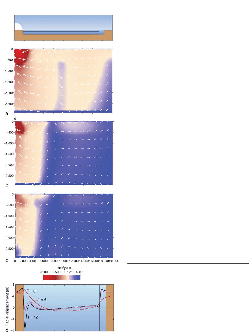
This is illustrated in Figure G38 for a simplified model in

which the ice sheet, land mass, and ocean basin are longitude

independent. In this case, a continent-based ice sheet at the

north pole, with dimensions approximating the North American

Ice Sheet, has been rapidly removed and only the rates of man-

tle displacement caused by the changing ice loads are shown

for three epochs, 100 years after the unloading, and 6,000

and 12,000 years later. The deformation extends throughout

the mantle, down to the core-mantle boundary at ~2,900 km

depth, and to the antipodes of the ice cap. The contribution to

this deformation field from the water loading is much smaller

in amplitude and this is shown here only as the radial displace-

ment of the sea surface for three epochs, immediately after

unloading and showing the elastic deformation, and at 6,000

and 12,000 years later. These signals, while relatively small,

are observationally significant and important for estimating

the mantle rheology, particularly at margins far from the former

ice sheets, such as across the antipodal margin illustrated.

GLACIAL ISOSTASY 375

If the parameters defining the Earth’s response function (its

rheology) are only partly known, then the comparison of pre-

dictions with observations provides a means of estimating this

function. If the ice history, the location and thickness of ice

through time, is not fully known then such a comparison may

contribute to the description of the past ice sheets. In fact,

neither the rheology nor ice history are perfectly known and

the primary motivation for the study of glacial isostasy is to

better understand the solid planet’s response to stress in support

of dynamical planetary studies, and to improve the description

of the past ice sheets in support of palaeoclimate studies.

As sea level rises and falls, it leaves behind signals of its

past position. Submerged terrestrial materials, such as in-situ

tree stumps, indicate that sea levels were lower at the time of

tree growth than today. Coral reefs above present sea levels

are indicative of sea levels having been higher in the past.

Thus, if the age of the tree stump or of the coral can be mea-

sured, limiting values to past sea levels can be established. In

some instances, high resolution observations are possible. The

submerged sediments may contain faunal or floral fossils

of species that lived only in a narrow tidal range or the mor-

phology of the reef may indicate that it formed at the upper

growth limit of corals. In either case, the paleoshoreline

can be precisely identified. Some examples of results from dif-

ferent parts of the world are illustrated in Figure G39 and these,

for the period since the Last Glacial Maximum (LGM)

at ~30,000–20,000 years ago, reveal some of the principal

spatial variabilities of the sea-level signal.

The results for Ångermanland, northern Sweden, and

Richmond Gulf, Canada, are characteristic for locations that

are near the former centers of glaciation, where the dominant

contribution to the relative sea-level change is from the crustal

rebound upon removal of the ice. Note that in the Swedish

example, the last ice disappeared about 9,000 years ago but since

then more than 200 m of rebound has occurred, testimony to the

viscous relaxation of the mantle. The example from the Norwe-

gian coast at Andøya is characteristic of the sea-level signal from

near ice margins. A similar result is observed at Vestfold Hills in

Antarctica, although the early part of the record here does not

appear to have been preserved in the sediments, or deglaciation

occurred late. The result from the Bristol Channel is representa-

tive of areas beyond but not far from the ice margins and here

sea levels have not been higher than present at any time since

the LGM. Similar signals are seen along the North American

Atlantic coast south of around New York. The observations from

Figure G38 Mantle deformation as the result of glacial loading at one

pole. The model is axisymmetric about the pole of the ice sheet, which

rests on a continent of the same dimension (left hand side, top panel).

A second, unloaded continent occurs at the antipodes (right hand side).

The ice sheet is assumed to melt instantaneously and the water is

added into the ocean basin between the two continents. The panels

(a–c) illustrate the rates of displacement of mantle material at three

epochs: (a) soon after the unloading and upon completion of the elastic

response, (b) 6,000 years after unloading, and (c) 12,000 years after

unloading. The arrows indicate the direction of flow and their lengths are

proportional to the magnitude of the flow rate on a logarithmic scale.

The color coding indicates the magnitudes of the rates. Panel (d) gives

the radial displacement of the ocean surface immediately after melting

(at time T =0

) and at 6,000 and 12,000 years ago (T = 6, 12 ka) due to

the addition of the water load into the ocean basin.

376 GLACIAL ISOSTASY