Pugnaire F.I. Valladares F. Functional Plant Ecology

Подождите немного. Документ загружается.

(ABA), which mediates stomatal closure (Davies and Zhang 1991). When soil water is not

limited, and when the internal CO

concentrations fall below ambient levels in the atmosphere,

stomata opens in sunlight. In approximately half of the known species, stomata have the

additional capability of sensing the relative humidity (RH) of the ambient air and tend to

progressively close as RH in the air adjacent to the leaves decreases. Rapid stomatal opening is

mediated by movement of K

from the epidermal cells to the guard cells (Figure 6.2c–f ). The

movement of K

makes p

less negative in the epidermal cells and more negative in the guard

cells; consequently, water flows from the epidermal cells to the guard cell, P

falls in the epidermal

Guard cell

Subsidiary cell

Epidermal cell

Closed stomate

Open stomate

Vein

Cuticle

Palisade

Mesophyll

Lower

epidermis

Guard cell

Upper

epidermis

(d)(c)

(f)

(a)

(b)

(e)

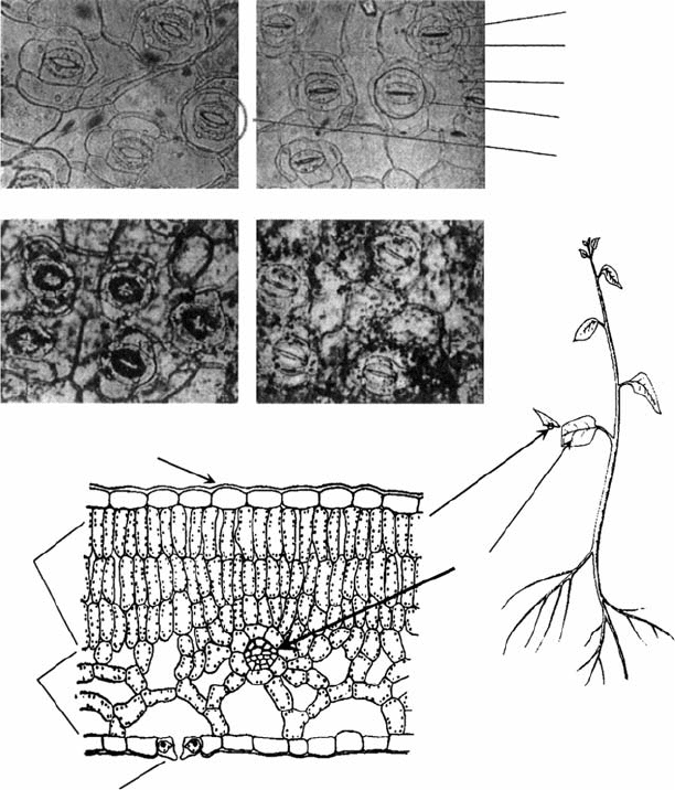
FIGURE 6.2 (a) A typical plant. (b) The lower leaf has been cut and the cross section is shown enlarged

approximately 750. (c–f ) Photographs of the lower leaf surface enlarged approximately 1000. (e) and

(f ) have been stained to show location of K

. (c) and (e) illustrate the open state of stomata when the

leaf is exposed to light. Stoma is from the Greek and means mouth (plural, stomata); the two guard cells

for a structure looks much like a mouth. (d) and (f ) are similar leaves in light but also exposed to abscisic

acid (ABA), causing stomata to remain closed in light. Note that in open stomata, K

is concentrated in

the guard cells (e) and the guard cells have moved apart to form an air passage for gas exchange (the

stomatal pore). Note that the K

is located in the epidermal cells when the stomata are closed

(f ). (Adapted from Kramer, P.J., Water Relations of Plants, Academic Press, New York, 1983; Bidwell,

R.G.S., Plant Physiology, Macmillan, New York, 1979.)

Francisco Pugnaire/Functional Plant Ecology 7488_C006 Final Proof page 180 10.5.2007 2:47pm Compositor Name: VBalamugundan

180 Functional Plant Ecology

cells, and P

rises in the guard cells. The mechanical effect of this water movement and change in

causes the guard cells to swell into the epidermal region and open a stomatal pore.

The evaporative flux density (E) of water vapor from leaves is ultimately governed by

Fick’s law of diffusion of gases in air. The control exercised by the plant is to change the area

available for vapor diffusion through the opening and closing of stomatal pores. The value of

E (mmol water s

1

2

of leaf surface) is given by

E ¼ g

 X

), (6:8)

where g

is the diffusional conductance of the leaf (largely controlled by the stomatal

conductance, g

), X

is the mole fraction of water vapor at the evaporative surface of the

palisade and mesophyll cells, and X

is the mole fraction of water vapor in the ambient air

surrounding the leaf. The mole fraction is defined as X ¼n

=N, where n

is the number of

moles of water vapor and N is the number of moles of all gas molecules, including water

vapor, the most abundant gas molecules are N

and O

. The dependence of g

on some

environmental and physiological variables is illustrated in Figure 6.3.

The maximum value of X occurs when RH is 100%, that is, when the air is saturated with

water vapor; the maximum value of X increases exponentially with the Kelvin temperature of

the air. The air at the evaporating surface of leaves is at the temperature of the leaf (T

), and

is taken as the maximum value of X at saturation, which can be symbolized as X

¼X [T

(a)

01234−2.5 −2.0 −1.5 −1.0 −0.5 0.0

⌿

(MPa)V

(kPa)

500

1.0

0.8

0.6

0.4

0.2

0.0

1.0

0.8

0.6

0.4

0.2

0.0

1000

PAR (µE m

−2

−1

)

(°C)

Relative g

1500 2000 0 15 20 25 30 35

(b)

(d)(c)

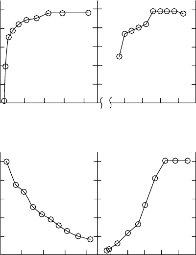
FIGURE 6.3 Relationship between change of g

relative to the maximum value, g

L,max

, and various

environmental factors measured on Acer saccharum leaves. The environmental factors were: (a) photo-

synthetically active radiation (PAR), (b) leaf temperature (T

), (c) vapor pressure deficit (V

), and

(d) leaf water potential (C

). (Adapted from Yang, S., Liu, X., and Tyree, M.T., J. Theor. Biol., 191,

197, 1998. With permission.)

Francisco Pugnaire/Functional Plant Ecology 7488_C006 Final Proof page 181 10.5.2007 2:47pm Compositor Name: VBalamugundan

Water Relations and Hydraulic Architecture 181

The value of X

depends on the microclimate near the leaf, that is, the air temperature and

RH. However, the microclimate of the leaf is strongly influenced by the behavior of the plant

community surrounding the leaf. Therefore, although the leaf has direct control over the

value of g

and g

, it has less control over E than might appear from Equation 6.8.

The qualitative aspects of how leaves influence their own microclimate is easily explained.

When the sun rises in the morning, the radiant energy load on the leaf increases. This has two

effects: T

rises as the sun warms the leaves, and hence, X

rises and g

increases as stomata

open. However, the increased evaporation from the leaves causes X

to rise as all the water

vapor is added to the ambient air. Even changes of g

under constant radiant energy load

causes less change in E than might be expected from Equation 6.8. When g

doubles, E also

doubles, but only temporarily. The increased E lowers T

because of increased evaporative

cooling, and hence lowers X

. The increased E from all of the leaves in a stand eventually

increases X

, hence X

X

declines, causing a decline in E. Consequently, Equation 6.8 is not

very useful in predicting the value of E at the level of plant communities. Leaf-level behavior

can be extrapolated to community-level equations if we take into account leaf-level solar

energy budgets, that is, equations that describe light absorption by leaves at all wavelengths

and the conversion of this energy to temperature and heat fluxes. Studies of solar energy

budgets have been conducted at both the leaf and stand-level (Slatyer 1967, and Chang 1968;

see also Section ‘‘Factors Controlling the Rate of Water Uptake and Movement’’).

Most of the changes in E at the leaf level can be explained in terms of net radiation

absorbed at the stand level, which is relatively easy to measure. This relationship is illustrated

in Figure 6.4, where daily values of E at the leaf level (kg m

2

day

1

) are correlated with daily

0.0

0.5

1.0

1.5

2.0

Bp (9)

Fm (1)

Ip (2)

Cs (4)

Cd (3)

Pa (4)

Bf (2)

Da (2)

246

∗

(kg m

−2

day

−1

)

Net radiation (MJ m

−2

day

−1

)

8101214

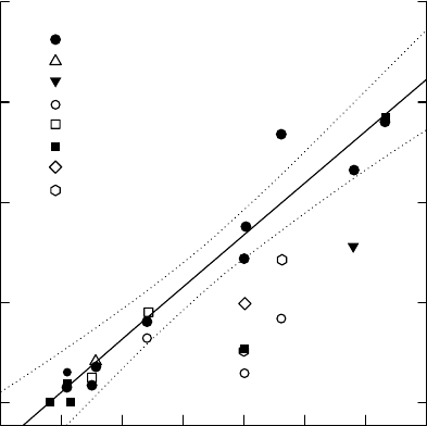
FIGURE 6.4 Correlation of daily water use of leaves (E*) and net radiation (NR). Data are from

potometer experiments with nine woody cloud forest species in Panama. The number of days per species

is given in parenthesis. The regression (with 95% confidence intervals) is for Bp: Baccharis pendunculata

(E* ¼0.20 þ1.29 NR, r

¼0.92). Even when the data for all species are pooled, NR proved to be a very

good predictor of daily water use (E* ¼0.2 þ1.04 NR, r

¼0.72). Cm, Citharexylum macradenium; Cd,

Croton draco; Fm, Ficus macbridei; Ip, Inga punctata; Pa, Parathesis amplifolia; Bf, Blakea foliacea; Cs,

Clusia stenophylla; and Da, Dendropanax arboreus. (From Zotz, G., Tyree, M.T. Patin

o, S., and

Carlton, M.R., Trees, 12, 302, 1998. With permission.)

Francisco Pugnaire/Functional Plant Ecology 7488_C006 Final Proof page 182 10.5.2007 2:47pm Compositor Name: VBalamugundan

182 Functional Plant Ecology

values of net radiation (MJ m

2

of ground per day) measured with an Eppley-type net

radiometer. Equations presented elsewhere to describe stand-level E in terms of net radiation

and other factors are validated by relationships such as shown in Figure 6.4. The other factors

most commonly included account for plant control over E through leaf area index (leaf area

per unit ground area), the effect of drought on g

, and ambient temperature (see Section

‘‘Factors Controlling the Rate of Water Uptake and Movement’’).

TISSUE–WATER RELATIONS (PRESSURE–VOLUME CURVES)

From the preceding section, the reader might falsely conclude that plants can lose water

from leaves without any negative impact on the growth and survival. However, there is

more to water loss than is apparent from stomatal physiology and the energy interactions

between leaves and their immediate environment. Whenever leaves lose water faster than the

rate of water uptake by roots, the water potential in the xylem (C

) and of the leaf cells (C

)

must also fall (see Section ‘‘Water Relations of Plant Cells’’). Most of the decline in C

due to a drop in P

, and when P

becomes too negative, cavitations occur that prevent water

flow through vessels (see Section ‘‘Cohesion–Tension Theory and Xylem Dysfunction’’).

Most of the decline in C

is due to a drop in P

, and when P

becomes too small, cell growth

stops. Growing cells are surrounded by relatively ridged ‘‘wooden boxes’’ consisting of

cellulose cell walls. Cell walls must be stretched plastically to grow large, and the motive

force on plastic stretch is the force of P

against the cell walls. As leaves lose water, P

and

must fall for the plant to extract water from the soil at a rate approximately equal to the

rate of water loss. As soils become dry, values of P

and P

must fall even more for plants

to extract water from soils. From Equation 6.7 it can be seen that P

¼C

p

, hence

plants have some control over P

through ‘‘adjustments’’ in p

. Some species have evolved

to have lower values of p

than others, and some species can make p

more negative in

response to drought by increasing the osmolal concentration (C) of solutes in their cells

(because p

¼RTC).

The relationship between C and its components (P and p) in leaves can be described by a

leaf-level Ho

fler diagram (Figure 6.2a). Many studies have reported the comparative physi-

ology of tissue–water relationship of leaves and have discussed how differences in these

relationships might explain ecological adaptation of plants. Readers interested in learning

more should consult the references contained in Tyree and Jarvis (1982). The following is a

brief overview of how Ho

fler diagrams are measured in leaves and some ecological applica-

tions of this information.

The fastest way to derive a Ho

fler diagram is to measure the water potential of leaves

leaf

) versus water loss using a Scholander–Hammel pressure bomb (Scholander et al. 1965,

Tyree and Hammel 1972). This is done by obtaining a series of balance pressure (P

) versus

weight loss of leaves or shoots; the P

is an approximate measure of the C

leaf

. The pressure

bomb is a metal chamber into which is placed an excised leaf or shot (Figure 6.5a) that is at an

unknown water potential, C

leaf

. When gas pressure (P

gas

) is applied to the leaf surface, the

pressure of the fluid in the cells is increased by an equal amount so that

leaf

¼ C

¼ p

þP

gas

. The xylem water potential and cell water potential are at equili-

brium, C

¼C

; from this it follows that p

þP

¼p

þP

gas

or P

¼p

þP

gas

p

When the P

gas

is at the balance pressure (P

), P

has risen to zero and xylem sap is squeezed

out of the end of the branch or petiole protruding outside the pressure bomb (Figure 6.5).

Therefore, we have P

¼(p

þP

) þp

¼C

leaf

, when the branch or leaf was outside the

bomb) þp

¼P

. P

is usually approximated by C

leaf

since p

is usually much smaller than

leaf

. However, P

really measures P

and the pressure bomb cannot measure pressure

gradients within a leaf because all gradients dissipate during the P

measurement. In some

cases these distinctions are important to remember.

Francisco Pugnaire/Functional Plant Ecology 7488_C006 Final Proof page 183 10.5.2007 2:47pm Compositor Name: VBalamugundan

Water Relations and Hydraulic Architecture 183

0.5 0.6 0.7 0.8 0.9 1.0

0.0

−4

−3

−2

−1

0.3

0.6

Pressure

gauge

Pressure

release valve

Connected to

compressed

air source

Pressure

bomb

(a)

(b)

1/P

(MPa

−1

)

Water potential or components (MPa)

(MPa)

0.9

1.2

1.5

⌿

␲

6 8 10 12

∆W (g)

14 16 18 20 22 24

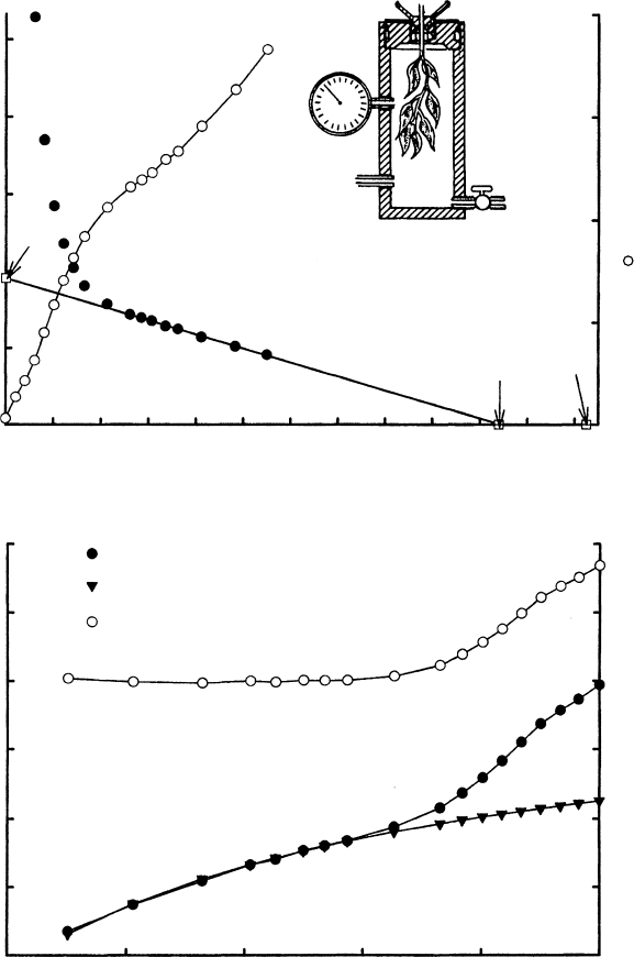
FIGURE 6.5 Scholander–Hammel pressure bomb and analysis of pressure bomb data. (a) A pressure

bomb is shown in the inset. Open circles (right axis): Original data of balance pressure (P

) versus weight

loss of shoot in the bomb. Weight loss is induced by removing the shoot from the bomb and allowing

water to evaporate. Closed circles (left axis): Transformed data of 1=P

versus weight loss. The liner

portion of the curve has been extrapolated to two points, A ¼y-intercept ¼1=p

, where p

is the

average osmotic pressure of the symplast at full hydration when C ¼0; B ¼x-intercept ¼weight of water

in the symplast when C ¼0 [this value can also be computed from (1=p

)=slope]; C ¼total

water content of the shoot ¼maximum weight loss when oven-dried. (b) The Ho

fler diagram for the

whole shoot derived from the data in (a). The x-axis is relative water content of the shoot and the y-axis

is p ¼osmotic potential of the symplasm (solid triangles), P

¼turgor pressure of symplasm (open

circles), and C ¼total water potential of the symplasm (solid circles).

Francisco Pugnaire/Functional Plant Ecology 7488_C006 Final Proof page 184 10.5.2007 2:47pm Compositor Name: VBalamugundan

184 Functional Plant Ecology

A pressure–volume curve is obtained by slowly dehydrating a shoot and obtaining a series

of weights, W, versus P

values. If W

was the original weight, then the cumulative weight

loss is DW ¼W

W. The pressure–volume curve is a plot of 1=P

versus DW. Strictly

speaking, the pressure–volume curve should be called a pressure–weight curve, but if DW is

given in g, then that is the same as volume in mL since 1 mL of water weighs 1 g. The

pressure–volume curve has a curved region for small DW values and a linear region for larger

DW values (Figure 6.5b). When the linear portion of the plot is extrapolated back DW ¼0, the

y-intercept (the point marked A in Figure 6.5a) is equal to 1=p

, where p

is the solute

potential of the living cells at zero water potential. The point marked B in Figure 6.5a is the

turgor loss point (C

tlp

), that is, the value of C

leaf

when P

reaches zero. The x-intercept

(point C) is the volume of water contained in the symplast (W

¼total water in the proto-

plasm and vacuoles of all living cells), and the difference in x-values (D–C) is the amount of

water in the apoplast (W

¼total water in xylem and cell walls). Ho

fler diagrams for shoots or

leaves are usually plots of C, p, and P

versus relative water content of the shoot or leaf.

Relative water content (R

) is defined as (the current water content)=(the maximum water

content at full hydration), R

¼(W

DW )=(W

W

), where W

is the dry weight. Values

of p at different R

are calculated from p

=(W

DW ), values of C are equated to

P

, and values of P

are calculated from P

p

. The justification for these relation-

ships is given in a report by Tyree and Hammel (1972).

As plants dry, changes in p can be caused by changes in symplastic water content, W

,orin

the number of moles of solute in the symplasm, N

, because p ¼RTN

. Considerbale

emphasis has been placed on demonstrating changes in p as a result to changes in N

(Turner

and Jones 1980). A change in p caused by a change in N

is called an osmotic adjustment.

Diurnal changes in p ranging from 0.4 to 1.6 MPa have been reported for some plants; the

amount of change resulting from diurnal changes in N

is in the range of 0.2–0.8 MPa. Medium-

term changes in p induced by slow soil dehydration have also been attributed to osmotic

adjustment in drought-stressed versus unstressed plants. Osmotic adjustments of 0.1–1 MPa

have been reported over periods of 3 days to 3 weeks. Long-term or seasonal changes in p range

from 0.2 to 1.8 MPa; some of the largest changes are recorded during the onset of winter in

temperate plants and appear to be correlated to changes in frost tolerance. The degree of

diurnal, medium-term, and long-term osmotic adjustment varies widely between species.

There are some species that have shown little or no adjustment (Tyree and Jarvis 1982).

Low values of p in plants should enhance the ability of plants to take up soil water under

dry or saline conditions (Tyree 1976). This advantage is probably marginal in sandy soils

because the available water reserves at soil water potentials less than 0.4 MPa are very

small; therefore, the plant’s ability to grow deep roots (Section ‘‘Cohesion–Tension Theory

and Xylem Dysfunction’’) is probably of greater advantage. In clay soils, however, there are

considerable water reserves at water potentials less than 0.4 MPa, so that low leaf and root

values of p may be as important as root growth in assisting water uptake. Low values of p in

leaves also enable P

to remain above zero at lower values of C than otherwise would be

possible as C falls. This allows the maintenance of open stomata with larger apertures and

high stomatal conductances and higher net rates of photosynthesis down to lower values of C

than would be the case if p were higher (less negative). Osmotic adjustments and=or lower p

values also enable maintenance of turgor pressure for growth, since it has been shown that the

rate of volume growth (r ¼dV=dt) of a cell is given by m(P

Y ), where m is the growth rate

constant of a cell and Y is the yield point of the cell (Green et al. 1971).

Some attention in the past has been focused on the slope of the P

line in the Ho

fler

diagram in which the x-axis is R

. The bulk modulus of elasticity of a tissue is defined as

« ¼

: (6:9)

Francisco Pugnaire/Functional Plant Ecology 7488_C006 Final Proof page 185 10.5.2007 2:47pm Compositor Name: VBalamugundan

Water Relations and Hydraulic Architecture 185

The higher value of « represents higher value of the slope of P

versus R

. A large value of « is

seen as an advantage for water conservation. For a plant to extract water from the soil, it must

first lose some water so that its C

leaf

falls below the soil water potential. Because most of the

change in C

leaf

is due to the change in P

, a large value of « means that a plant would have to

lose less water to lower C

leaf

than would a plant with a small value of «.

Although values of « have been reported to range from 0.5 to 20 MPa, the adaptive

advantages of large versus small « have never been clearly established (Tyree and Jarvis 1982)

because the ecological advantage of a large « may be rather marginal. All plants lose water

during the day and regain most or all of the lost water during the night. Therefore, the

advantage of less water loss means more constant concentrations of biochemical substrates

during the day. Leaves can lose anywhere from 1% to 20% of their water content during the

day, and this water loss would cause a corresponding 1%–20% diurnal variation in substrates.

Because the concentration of reactants and products would normally change during the day,

even without the influence of leaf dehydration, it is not clear how much is gained by keeping

relatively constant cell volume because of large «.

WATER ABSORPTION BY PLANT ROOTS

The primary factor affecting the pattern of water extraction by plants from soils is the rooting

depth. Rooting depths can be extremely variable depending on soil conditions and species of

plant producing the roots (Figure 6.6a). Many of the early studies of rooting depth and

branching pattern of roots were performed in the 1920s and 1930s in deep, well-aerated

prairie soils, where roots penetrate to great depths. At the extreme, roots have been traced to

depths of 10–25 m, for example, alfalfa (10 m), longleaf pine, (17 m) (Kramer 1983), and

drought-evading species in the California chaparral (25 m) (S. Davis, April 1991, personal

communication). The situation is very different for plants growing in heavy soils, where 90%

of the roots can be found in the upper 0.5–1.0 m.

In seasonally dry regions, for example, central Panama, the majority of the roots may be

located in the upper 0.5 m, but it is far from clear if the majority of water absorption occurs in

the upper 0.5 m during the dry season. Water use by many evergreen trees is higher in the dry

season than in the wet season, although the upper 1 m of the soils is much drier than the leaves

of the trees (C

soil

< C

leaf

) and excavations have shown that liana roots are less than 5 m in

depth and hence extract water from quite wet soil during the dry season (M.T. Tyree,

February 1989, personal observation). Hence, the role of shallow versus deep roots of

woody species deserves more study.

In addition, deeply rooted species may contribute to the water supply of shallow-rooted

species through a process called hydraulic lift (Richards and Caldwell 1987). In one study, it

was found that shallow-rooted species growing within 1–5 m of the base of maple trees were in

a better water balance than the same species growing more than 5 m away (Dawson 1993).

Each night, the C

soil

at a depth of 0.5 m increased underneath maple trees, but C

soil

did not

increase at distances greater than 5 m from the trees. This indicated that the deep maple roots

were in contact with moist soil and were capable of transporting water from deep maple

roots to shallow maple roots overnight. Since the water potential of the shallow maple roots

exceeded the water potential of the adjacent soil, water flow from the shallow maple roots to

the adjacent soil contributed to the overnight rehydration of shallow soils.

Roots absorb both water and mineral solutes found in the soil, and the flow of solutes and

water interact with each other. The mechanism and pathway of water absorption by roots is

more complex than in the case of a single cell (Section ‘‘Water Relations of Plant Cells’’).

Water must travel first radially from the epidermis to cortex, endodermis, and pericycle

before it finally reaches the xylem vessels, from which point water flow is axial along

Francisco Pugnaire/Functional Plant Ecology 7488_C006 Final Proof page 186 10.5.2007 2:47pm Compositor Name: VBalamugundan

186 Functional Plant Ecology

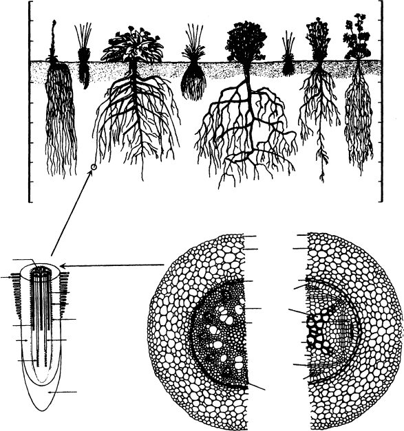
the root (Figures 6.6b and 6.6c). The radial pathway (typically 0.3 mm long in young roots) is

usually much less conductive than the axial pathway (>1 m in many cases); therefore,

whole-root conductance is generally proportional to the root surface area. The radial

pathway can be viewed as a composite membrane separating the soil solution from the

solution in the xylem fluid. The composite membrane consists of serial and parallel pathways

made up of plasmalemma membranes, cell wall ‘‘membranes,’’ and plasmodesmata

(pores <0.5 mm diameter) that connect adjacent cells. The composite membrane is rather

leaky to solutes; therefore, differences in osmotic potential between the soil (p

) and the xylem

) have less influence on the movement of water. At any given point along the axis, the

water flux density across the root radius (J

) is given by

¼ L

[(P

 P

) þ s(p

 p

)], (6:10)

(a)

(c)

(b)

0.6

0.0

0.6

1.2

1.8

Immature

metaxylem

Immature

protoxylem

Immature

protophloem

Root hair

Root cap

Protophloem

Pericycle

Protoxylem

Epidermis

Cortex

Endodermis

Pericycle

Xylem

Phloem

Monocot Dicot

Parenchyma

Primary xylem

Secondary

xylem

Cortex

Endodermis

FIGURE 6.6 (a) Differences in root morphology and depth of root systems of various species of prairie

plants growing in a deep, well-aerated soil. Species shown are: h, Hieracium scouleri;k,Loeleria cristata;

b, Balsamina sgittata;f,Festuca ovina ingrata;g,Geranium viscosissimum;p,Poa sandbergii; ho,

Hoorebekia racemosa; and po, Potentilla blaschkeana. (b) Enlargement of a dicot root tip enlarged

approximately 50. (c) Cross section of monocot and dicot roots enlarged approximately 400.

(Adapted from Kramer, P.J., Water Relations of Plants, Academic Press, New York, 1983; Steward,

F.C., Plants at Work, Addison-Wesley, Reading, MA, 1964; Bidwell, R.G.S., Plant Physiology,

Macmillan, New York, 1979.)

Francisco Pugnaire/Functional Plant Ecology 7488_C006 Final Proof page 187 10.5.2007 2:47pm Compositor Name: VBalamugundan

Water Relations and Hydraulic Architecture 187

where L

is the radial root conductance to water and s is the solute reflection coefficient. For

an ideal membrane in which water but not solutes may pass, s ¼1. For the composite

membrane of roots, s is usually between 0.1 and 0.8. The system of equations that describes

water transport in roots is complex when all of the factors are taken into account, for

example, axial and radial conductances, the fact that each solute has a different s, and that

the rate of water flow is influenced by the solute loading rate (J

). Water and solute flow in

roots can be described by a standing gradient osmotic flow model (readers interested in the

details may consult Tyree et al. (1994b) and Steudle (1992).

Fortunately, the equations describing water flow become simple when the rate of water

flow is high. The concentration of solutes in the xylem fluid is equal to the ratio of solute flux

to water flux (J

) during steady-state flux. Solute flux tend to be more or less constant with

time, but water flux increases with increasing transpiration. When water flow is high, the

concentration of solutes in the xylem fluid becomes small and approaches values comparable

to that in the soil solution, and pressure differences become quite large, hence (P

P

) >>

p

). Only at night or during rainy periods can values of (P

P

) approach those of

s(p

p

). Therefore, water flow (J

,kgs

1

) through a whole-root system during the day can

be approximated by

ﬃ k

P

x,b

)(6:11)

where P

x,b

is the xylem pressure at the base of the plant and k

is the total root conductance

(combined radial and axial conductances).

HYDRAULIC ARCHITECTURE AND PATHWAY OF WATER

MOVEMENT IN PLANTS

Van den Honert (1948) quantified water flow in plants in a classical paper in which he viewed

the flow of water in the plant as a catenary process, where each catena element is viewed as a

hydraulic conductance (analogous to an electrical conductance) across which water (analogous

to electric current) flows. Thus, van den Honert proposed an Ohm’s law analog for water flow

in plants. The Ohm’s analog leads to the following predictions; (1) the driving force of sap

ascent is a continuous decrease in P

in the direction of sap flow; and (2) evaporative flux

density from leaves (E) is proportional to negative of the pressure gradient (dP

=dx) at any

given point (cross section) along the transpiration gradient (dP

=dx) at any given point

(cross section) along the transpiration stream. Thus, at any given point of a root, stem, or leaf

vein, we have

dP

=dx ¼ AE=K

þ rg dh=dx, (6:12)

where A is the leaf-area supplied water by a stem segment with hydraulic conductivity K

and rg dh=dx is the gravitational potential gradient, where r is density of water, g is acceler-

ation due to gravity, and dh=dx is height gained, dh, per unit distance, dx, traveled by water in

the stem segment.

In the context of stem segments of length (L) with finite pressure drops across ends of the

segment, we have

¼ LAE=K

þ rgDh: (6:13)

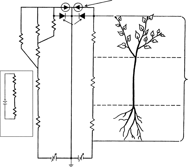
Figure 6.7 illustrates water flow through a plant represented by a linear catena of conductance

elements near the center and a branched catena of conductance elements on the left. The

number and arrangement of catena elements are dictated primarily by the spatial precision

Francisco Pugnaire/Functional Plant Ecology 7488_C006 Final Proof page 188 10.5.2007 2:47pm Compositor Name: VBalamugundan

188 Functional Plant Ecology

desired in the representation of water flow through a plant; a plant can be represented by

anywhere from one to thousands of conductance elements. Reviews of the hydraulic archi-

tecture of woody plants can be found in a report by Tyree and Ewers (1991 and 1996).

The usual way of representing the Ohm’s law circuit is incomplete. The usual but

incomplete representation of the Ohm’s law circuit is shown in the boxed inset in the lower

left side of Figure 6.7. The battery represents the water potential drop from root to leaf, but it

is an incomplete representation of reality because no ground point is shown in the circuit. The

ground point represents zero water potential. Water potential is always measured relative to

pure water at the same temperature and pressure as the plant. The incomplete representation

gives the correct drop in water potential across each conductance element but not the correct

water potential relative to ground (the zero reference). The complete representation has a

variable battery that gives the soil water potential (C

soil

) and has some analog components to

represent the evaporation from the leaves. In Figure 6.8, the evaporation is shown by a constant

current source and a rectifier in parallel. The amount of current, E, in the constant current

source can be approximated by Equation 6.8. When E ¼0 we expect leaf water potential to

equal soil water potential and that there should be no water current flowing through the

circuit; this condition is achieved in the circuit by the introduction of the rectifier that

prevents backward current flow when E ¼0andC

soil

< 0. In some experimental conditions,

soil

can be raised to positive values by placing a potted root system in a pressure chamber with

Branched model

Usual

incomplete

representation

−−++

leaf 2

leaf1

leaf

stem 2

stem1

stem

liquid

stem

root

⌿

soil

⌿

soil

⌿

root

⌿

leaf

⌿

soil

root

leaf 3

leaf

Rectifier

−0.7 (MPa)

−0.2 (MPa)

−0.05 (MPa)

Linear

model

(constant current source)

= g

∆X

FIGURE 6.7 The Ohm’s law analogy. The total conductance is seen as resultant conductance (K ) of the

root, stem, and leaf in series and parallel. Water flow is driven by evaporation of water from leaves,

which creates a difference in water potential between the soil, C

soil

, and the water potential at the

evaporating surface, C

evap

. On the right is the simplest Ohm’s law analogy with conductances in series.

On the left is a more complex conductance catena in which some conductance elements are in series and

some in parallel.

Francisco Pugnaire/Functional Plant Ecology 7488_C006 Final Proof page 189 10.5.2007 2:47pm Compositor Name: VBalamugundan

Water Relations and Hydraulic Architecture 189