Roy K.K. Potential theory in applied geophysics
Подождите немного. Документ загружается.


8.3 Potential for a Transitional Earth 239
Since
∂
2
φ
∂x
2
+
∂
2
φ
∂y
2
+
∂
2
φ
∂z
2
=
∂
2
φ
∂r
2
+
1
r
∂φ
∂r
+
∂
2
φ
∂z
2
(8.161)
when φ is independent of the azimuthal angle, hence (8.161) can be written
as
1
ρ (z)
∂
2
φ
∂r
2
+
1
r
∂φ
∂r
+
∂
2
φ
∂z
2
+
1
∂z
1
ρ (z)
∂φ
∂z
= 0 (8.162)
⇒
1
ρ (z)
∂
2
φ
∂r
2
+
1
r
∂φ
∂r
+
∂
2
φ
∂z
2
−
1
(ρ (z))
2
∂ρ
∂z
∂φ
∂z
=0
⇒
∂
2
φ
∂r
2
+
1
r
∂φ
∂r
+
∂
2
φ
∂z
2
−
ρ
′
(z)
ρ (z)
.
∂φ
∂z
=0. (8.163)
Applying the method of separation of variables and assuming φ(r
1
z) =
R(r)Z(z), we get
∂
2
φ
∂r
2
=
∂
2
R
∂r
2
Z(z)
∂
2
φ
∂z
2
=R(r)
∂
2
Z
∂z
2
∂φ
∂z
=R(r)
∂R
∂z
. (8.164)
Therefore
d
2
R
dr
2
Z(z)+
1
r
dR
dr
Z(z)+
d
2
Z
dz
2
R(r)−
ρ
′
(z)
ρ (z)
dZ
dz
R(r)=0
d
2
R
dr
2
Z(z)+
1
r
dR
dr
Z(z) =−
d
2
Z
dz
2
R(r)+
ρ
′
(z)
ρ (z)
.
dZ
dz
R(r)
⇒
1
R
d
2
R
dr
2
+
1
r
+
dR
dr
= −
d
2
Z
dz
2
−
ρ
′
ρ
dZ
dz
1
Z
= −λ
2
.
(8.165)
We get
d
2
R
dr
2
+
1
r
dR
dr
+ λ
2
R=0
⇒ r
2
d
2
R
dr
2
+r
dR
dr
+ λ
2
r
2
R=0. (8.166)
The second equation is
−
d
2
Z
dz
2
−
ρ
′
ρ
dZ
dz
+ λ
2
Z=0
⇒−
d
2
Z
dz
2
+
ρ
′
ρ
dZ
dz
+ λ
2
h=0
⇒ Z
′′
−
ρ
′
ρ
Z
′
− λ
2
h=0. (8.167)

240 8 Direct Current Field Related Potential Problems
Therefore, the general solution of the equation
φ (r, z)=
∞
0
A (λ) Z (z,λ)J
0
(λr) dx. (8.168)
Since
∂φ
∂z
at the air-earth boundary vanishes, we have.
∂φ
∂z
=
∞
0
A (λ) J
0
(λ, r)Z
′
(z,λ) dλ = 0 (8.169)
where
Z
′
(z, λ)=
dZ
dλ
.
We get
A(λ)=
B(λ)
Z
′
(0, λ)
.
Since
∞
0
λJ
0
(λr) dλ =0,φ(r
1
,z)=B
∞
0
λJ
0
(λr) k (z,λ) dλ (8.170)
where
κ (z, λ)=
Z(z, λ)
Z
′
(z, λ)
.
From homogeneous earth analogy, we get
B=
Iρ
0
2π
The solution of the equation is
φ (r, z) =
Iρ
0
2π
∞
0
λ
Z (z, λ)
Z
′
(0, λ)
.J
0
(λ, r) dλ. (8.171)
8.3.2 Potential for a Layered Earth with a Sandwitched
Transitional Layer
In this section, a three layer earth is assumed in which the second layer is
a transitio nal layer where σ = f(Z) (Fig. 8.5). Th e conductivity of the first
and second layer are respectively σ
1
and σ
3
. Thickness of the first a nd second
layer a re resp ectively h
1
and h
2
; thickness of the third layer is infinitely high.
Laplace equation is satisfied in the first and third layer. For the second layer
the non Laplacian governing equation is (Mallick a n d Roy, 1968).
8.3 Potential for a Transitional Earth 241
∇
2
φ +
1
σ
∂σ
∂z
.
∂φ
∂z
=0. (8.172)
In the transitional layer, the conductivity is assumed to vary linearly with
depth; so we get
σ = σ
1
+
σ
2
− σ
1
h
2
− h
1
(Z −h
1
) , (8.173)
σ = σ
1
at Z = h
1
and σ
2
at Z = h.
The guiding equations for solving the potential problems for the first,
second and third layers are r espectively given by
∇
2
φ
1
=0
∇
2
φ +
1
σ
∂σ
∂z
.
∂φ
∂z
=0
∇
2
φ
2
= 0 (8.174)
where φ
1
, φ and φ
2
are the potentials in the three regions
Here
φ
1
=q
∞
0
e
−mz
J
0
(mr) dm +
∞
0
A(m)
'
e
−mz
+e
mz
(
J
0
(mr) dm (8.175)
φ
2
=
∞
0
D(m)e
−mz
J
0
(mr)dm (8.176)
In the transitional zone
∂
2
φ
∂r
2
+
1
r
∂φ
∂r
+
∂
2
φ
∂Z
2
+
α
σ
1
+ α (z − h
1
)
∂φ
∂Z
= 0 (8.177)
where
α =
(σ
2
− σ
1
)
(h
2
− h
1
)
.
Fig. 8.5. A model of a three layer earth with middle layer as a transitional layer
242 8 Direct Current Field Related Potential Problems
Applying the method of separation of variables φ = R(r) Z (z), one gets,
dR
2
dr
2
+
1
r
dR
dr
+m
2
R = 0 (8.178)
and
d
2
Z
dz
2
+
α
σ
1
+ α (Z − h
1
)
dZ
dz
− m
2
Z=0. (8.179)
In the (8.179), we substitute
τ = σ
1
+ α(Z − h
1
).
One gets
dτ
dz
= α.
Therefore
dZ
dz
=
dZ
dτ
.
dτ
dz
= α
dZ
dτ
and (8.179) changes to the form
d
2
Z
dτ
2
+
1
τ
dZ
dτ
−
m
2
α
2
Z =0. (8.180)
The solution of (8.180) is
φ =
∞
0
(B (m) I
o
(mτ/α)+C(m)K
o
(mτ/α))J
o
(mr)dm. (8.181)
Now the constants A (m), B (m), C (m) and D (m) are to be evaluated from
the boun d ary conditions.
φ
1
= φ and
∂φ
1
∂Z
=
∂φ
∂Z
at Z = h
1
φ
2
= φ and
∂φ
∂Z
=
∂φ
2
∂Z
at Z = h
2
.
Applying the boundary conditions, we get
qe
−mh
1
+ A (m)
'
e
−mh
1
+ e
mh
1
(
= B (m) I
0
mτ
1
α
+ C (m) K
0
mτ
1
α
(8.182)
−qe
−mh
1
+ A (m)
'
−e
−mh
1
+ e
mh
1
(
= B (m) I
1
mτ
1
α
− C (m) K
1
mτ
1
α
(8.183)
D (m) e
−mh
2
= B (m) I
0
mτ
2
α
+ C (m) K
0
mτ
2
α
(8.184)
−D (m) e
−mh
2
= B (m) I
1
mτ
2
α
− C (m) K
1
mτ
2
α
(8.185)
8.3 Potential for a Transitional Earth 243
For surface geophysics, we are interested in A (m). It can be shown that
A(m)=
γ−1
γ+1
e
−2mh
1
1 −
γ−1
γ+1
e
−2mh
1
(8.186)
where
γ =
K
0
'
mσ
1
α
(
+ uI
0
'
mσ
1
α
(
K
1
'
mσ
1
α
(
− uI
1
'
mσ
1
α
(
here
u=−
K
0
'
mσ
2
α
(
+K
1
'
mσ
2
α
(
I
0
'
mσ
2
α
(
+I
1
'
mσ
2
α
(
.
Substituting the value of A (m) and putting z = 0, one gets the value of
potential at a point on the surface of the earth as
φ
1
(r, 0) =
I
2πσ
1
⎧
⎨
⎩
1
r
+2
∞
0
γ−1
γ+1
e
−2mh
1
1 −
γ−1
γ+1
e
−2mh
1
J
0
(mr)dm
⎫
⎬
⎭
. (8.187)
8.3.3 Potential with Media Having Coaxial Cylindrical Symmetry
with a Transitional Layer in Between
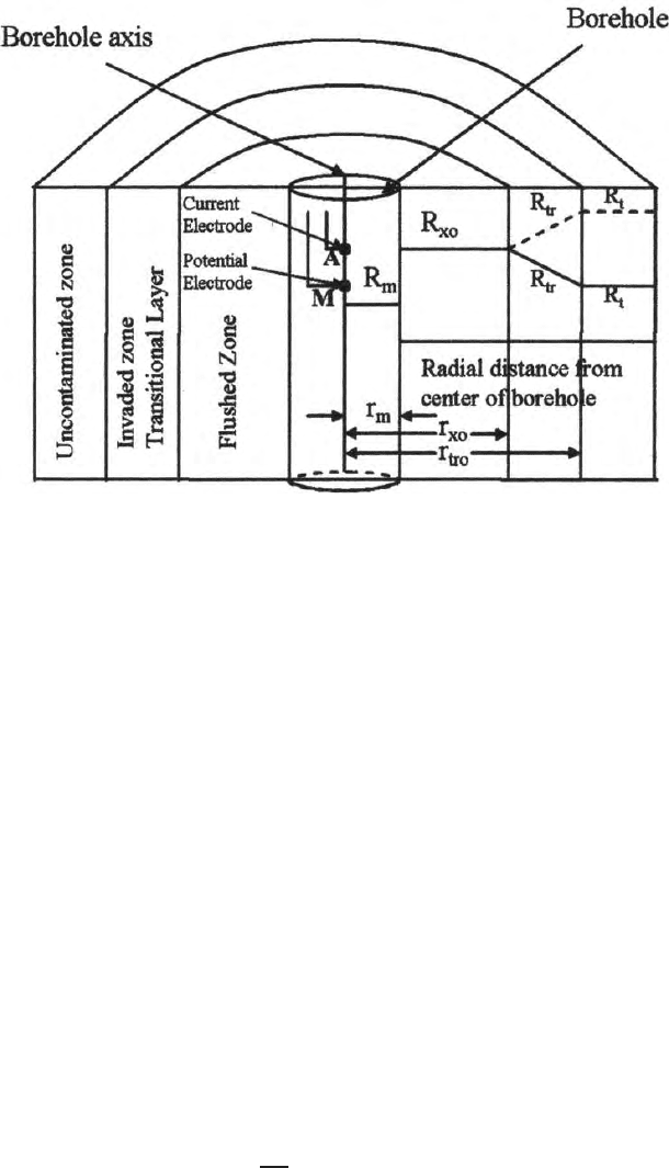
Figure (8.6) explains the geometry of the problem. In borehole geophysics
an one dimensional problem will have cylindrical boundaries. The maximum
numbers of layers generally created a re five. They include (i) bor ehole mud, (ii)
mud cake, (iii) flushed zone, (iv ) invaded zone and (v) uncontaminated zone.
Figure (8.6) explains the presence of these different zones. However the readers
should consult any text book on borehole geophysics to understand these well
logging terminologies. In borehole geometry, these layers are coaxial cylinders.
The effect of mud cake is negligible in the normal (two electrode) or lateral
(three electrode) log resp onse curves. Therefore, the problem is presented as
a four layer pr oblem. However, it can be extended to any number of layers.
(Dutta, 1993, Roy and Dutta 1994).This problem is presented to show that
a differential equa ti on, not having an easy solution, can be handled using
Frobeneous power series.
The problem is framed as a boundary value problem with a point sour ce
of current on the borehole axis having cylindrical coaxial layered media with
infinite bed thickness. Invaded zone is present as one of those layers as a
transitional zone where nonlaplacian term appears. Potentials satisfy Laplace
equation in all the homogenous and isotropic media where resistivities are
assumed to be constant.
Potential in the medium 1 (i.e. in the borehole) is given by
φ
1
=
R
m
I
2π
2
r
m
∞
0
K
0
(mr) cos mz dm +
∞
0
C
1
(m) I
0
(mr) cos mz dm. (8.188)
(Dakhnov, 1962) (Sect. 8 .2).
244 8 Direct Current Field Related Potential Problems
Fig. 8.6. A cross section of a borehole with transitional invaded zone
The first integral is a potential due to a point source. This expression is
obtained after applying the Weber Lipschitz identity. The second integral is
the perturbation potential. I
0
(mr) and K
0
(mr) are respectively the modified
Bessel functions of the first and second kind of order zero. Here the parameter
R
m
is the resistivity of the b orehole mud and r
m
is the radius of the borehole. m
is the integration variable, z is a point of observation in the assumed borehole,
r is the radial distance from the axis of the borehole. C
1
(m) is the kernel
function to be evaluated applying suitable boundary conditions. Potentials in
the second and fourth media are given by
φ
2
=
∞
0
C
2
(m) K
0
(mr) cos mz dm +
∞
0
C
3
(m) I
0
(mr) cos mz dm (8.189)
and
φ
4
=
∞
0
C
6
(m) K
0
(mr) cos mz dm. (8.190)
For φ
4
there is no integral involving I
0
(mr) which tend to become infinite for
large values of the argument r.
Potential in the transitional invaded zone is derived from,
φ
2
φ
3
+
1
σ
tr
grad σ
tr
grad φ
3
= 0 (8.191)

8.3 Potential for a Transitional Earth 245
where, σ
tr
is the conductivity of the transition zone and grad σ
tr
is non zero.
Simplification of the differential equation by a suitable substitution, like previ-
ous problems, was not possible in this case. Two different situations can exist
for the transition zone i.e., i) when R
t
< R
x0
and ii) R
t
> R
x0
.HereR
t
is the
resistivity ofthe uncontaminated zone or zone 4 and R
x0
is the resistivity of
the flushed zo ne or zone 2. Resistivities of these two zones are assumed to be
fixed. For these two cases, two different modes of solution are presented. In
the first case resistivity in the transition zone is varying linearly with radial
distance and in the second case conductivity has a linea r gradient with radial
distance as shown in Part I and Part II.
Part 1: Potential Function in Transition Zone where R
t
< R
x0
Since the potential is independent of the azimuthal angle, (8.191) reduces to
the form, taking σ
tr
=1/R
tr
.
∂
2
φ
∂r
2
+
1
r
∂φ
3
∂r
+
∂
2
φ
∂z
2
−
1
R
tr
∂R
tr
∂r
∂φ
3
∂r
= 0 (8.192)
where, R
tr
is the resistivity of the transition zo ne.
Applying the method of separation of variables, i.e., φ
3
= R (r) Z (z),
(8.192) reduces to
d
2
Z
dz
2
+m
2
Z = 0 (8.193)
and
d
2
R
dr
2
+
1
r
dR
dr
−
1
R
tr
dR
tr
dr
dR
dr
− m
2
R=0. (8.194)
Equation (8.194) can be modified assuming linear transition in the invaded
zone, i.e.,
R
tr
= R
x0
+
R
t
− R
x0
r
tr
− r
x0
(r − r
x0
) (8.195)
where, R
tr
, the resistivity of the transition zone or invaded zone is a function
of radial distance r. r
tr
and r
x0
are the radial distances of the boundaries
between (i) uncontaminated zone and invaded zone and (ii) invaded zone and
flushed zone, we write
R
tr
=a
1
+ αr
where, a
1
=R
x0
− αr
x0
and α =
R
t
−R
x0
r
tr
−r
x0
.
After a few steps of algebraic simplifications, (8.194) reduces to the form
d
2
R
dr
2
+
a
r(a+r)
dR
dr
− m
2
R=0. (8.196)
Here a (= a
1
/α) is a lso a constant. Equation (8.195) is solved by Frobenious
extended power series assuming

246 8 Direct Current Field Related Potential Problems
R=
∞
p=0
A
p
r
p+q
(8.197)
(Kreyszig, 1985; Ayres, 1972). In this case (8.194), at r = 0, the coefficient of
dR/dr is not analytic and the extended power series method is considered for
solution.
Equation (8.195) is rewritten as
r
2
R
′′
+arR
′′
+aR
′
− m
2
r
2
R −am
2
rR=0. (8.198)
Substituting the values of R
′′
,R
′
and R obtained from (8.197) and (8.198),
where R
′′
and R
′
are the second and first derivatives of R with respect to r,
one gets,
∞
p=0
(p + q) (p + q − 1) A
p
r
p+q
+a
∞
p=0
(p + q) (p + q − 1) A
p
r
(p+q−1)
+a
∞
p=0
(p + q) A
p
r
(p+q−1)
− m
2
∞
p=0
A
p
r
(p+q+2)
− am
2
∞
p=0
A
p
r
(p+q+1)
=0.
(8.199)
The normal procedure is to equate the smallest power of r to zero and taking
p = 0, we get
Aq(q − 1)A
0
+aqA
0
=0. (8.200)
Since a and A
0
are not zero, hence q has distinct double roots and both
of them are zero. In order to find out the generalised form of the expression
for the coefficient A
p
, we equate the coefficients of r
q+r−1
to obtain
(q + p − 1)(q + p − 2)A
p−1
+a(q+p− 1)(q + p)A
p
+a(q+p)A
p
− m
2
A
p−3
− am
2
A
p−2
=0. (8.201)
From (8.201), one gets
A
p
=
1
a(q+p)
2
'
m
2
A
p−3
+am
2
A
p−2
− (q + p − 1) (q + p −2) A
p−1
(
.
(8.202)
Since (8.196) can be solved by taking the solution in the form of a Frobe-
nious extended power series. One of the solutions will be the (8.197) provided
we can determine the coefficient A
p
. Since the indicial equation has two dis-
tinct roots, (8.194) must have a second solution.
R
2
=
∂R
1
∂q
(Ayres 1972, Kreyszig 1985)

8.3 Potential for a Transitional Earth 247
=
∂
∂q
)
r
q
∞
p=0
A
p
r
p
*
=r
q
ln r
∞
p=0
A
p
r
p
+r
q
∞
p=0
∂A
p
∂q
r
p
. (8.203)
Therefore, q = 0, the two solutions are
T
1
(m, r) = R
1
|
q=0
=
∞
p=0
A
p
r
p
(8.204)
T
2
(m, r) = R
2
|
q=0
=ln R
1
+
∞
p=0
K
p
r
p
(8.205)
where
K
p
=
∂A
p
∂q
.
(Ayres 1972, Kreyszig 1985)
The generalised expression for K
p
can be shown, after a few steps of simple
differentiation and algebraic simplification. Taking A
0
=1,weget
K
1
=
∂A
1
∂q
=
∂
∂q
)
−
q(q− 1)
a(q+1)
2
*
= −
1
a
(q + 1)
2q
2
− 1
− 2q (q − 1) (q + 1)
(q + 1)
4
. (8.206)
Therefore at q = 0
K
1
=1/a
and
K
2
=
∂A
2
∂q
= −
2
a(q+2)
3
am
2
+
q(q− 1)
a(q+1)
+
1
a(q+2)
2
)
−
1
a
(q + 1)
3q
2
− 2q
− q
2
(q −1)
(q + 1)
2
*
. (8.207)
At q = 0
K
2
= −
m
2
4
K
3
=
∂A
3
∂q
= −
2
a(q+3)
3
'
am
2
A
1
+m
2
A
0
− (q + 2) (q + 1) A
2
(

248 8 Direct Current Field Related Potential Problems
+
1
a(q+3)
2
'
am
2
K
1
− (q + 2) (q + 1) K
2
− (2q + 3) A
2
(
K
3
= −
1
a
m
2
27
+
1
a
m
2
12
. (8.208)
Generalised expression for the term K
p
for p ≥ 4 can be formed taking q = 0,
as
K
p
= −
2
ap
3
C
p
+
'
m
2
K
p−3
+ am
2
K
p−2
− (p − 1) (p − 2) K
p−1
−(2p −3) A
p−1
] /ap
2
(8.209)
where,
C
p
=
'
m
2
A
p−3
+am
2
A
p−2
− (p − 1) (p −2) A
p−1
(
.
Part 2: Potential Function an Borehole Transitional Earth Model
zone where R
t
> R
X0
In this parametric setup where R
t
> R
X0
the value of a in the (8.199) may
assume a zero value for certain value of r, and the coefficient of dR/dr becomes
zero. To avoid this a l gebraic singularity, conductivity is considered to vary
linearly in this model (R
t
> R
X0
) in case of transitional invaded zone.
Potential expression in the transition zone (8.194) can be expressed as
∂
2
φ
3
∂r
2
+
1
r
∂φ
3
∂r
+
1
σ
tr
∂σ
tr
∂r
∂φ
3
∂r
+
∂
2
φ
3
∂z
2
= 0 (8.210)
which is independent of the azimuthal angle. Applying the method of separa-
tion of variables, (8.210) reduces to
d
2
Z
dz
2
+m
2
z = 0 (8.211)
d
2
R
dr
2
+
1
r
dR
dr
+
1
σ
tr
dσ
tr
dr
dR
dr
− m
2
R=0. (8.212)
Equations (8.194) and (8.212) are same as there is no heterogeneity in the z
direction. Assuming linear transition in electrical conductivity in the transi-
tion zone i.e.,
σ
tr
= σ
x0
+
σ
t
− σ
x0
r
tr
− r
x0
(r −r
x0
) (8.213)
where, σ
tr
is the conductivity of the transition zone and a function of radial
distance. σ
t
and σ
x0
are the conductivity of the uncontaminated and the
flushed zones respectively.
We write σ
tr
=a
1
+ σr
where,
a
1
= σ
x0
− σr
x0