Samarskii A.A., Vabishchevich P.N. Numerical Methods for Solving Inverse Problems of Mathematical Physics

Подождите немного. Документ загружается.

236 Chapter 6 Right-hand side identiﬁcation

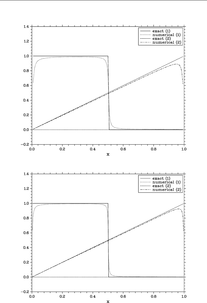
Figure 6.19 Solution of the problem obtained on the grid N

= N

= 129

Figure 6.20 Solution of the problem obtained on the grid N

= N

= 257

Section 6.6 Exercises 237

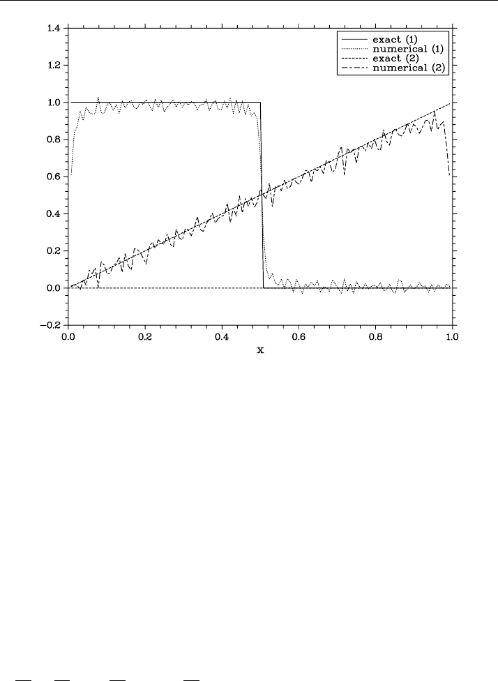
Figure 6.21 Solution of the problem obtained at the inaccuracy level δ = 0.0003

6.6 Exercises

Exercise 6.1 Formulate the condition for convergence of the approximate solution

determined from (6.16), (6.17), (6.19) to the solution of problem (6.14).

Exercise 6.2 Substantiate the iteration method (6.26) as applied to the approximate

solution of problem (6.14), (6.16).

Exercise 6.3 Modify the program PROBLEM5 so that to make it suitable for solving

the inverse problem (6.14), (6.16) by the iteration method (6.26). Give a comparative

analysis of the methods.

Exercise 6.4 Consider the basic speciﬁc features of the Tikhonov regularization

method as applied to solving the inverse problem on the identiﬁcation of the right-

hand side of parabolic equation with lower terms

∂u

∂t

∂

∂x



k(x)

∂u

∂x



+ b(x)

∂u

∂x

+ f (x, t), 0 < x < l, 0 < t ≤ T,

from a given function u(x, t).

Exercise 6.5 Construct an iterative local-regularization algorithm making it possible

to identify the right-hand side of the parabolic equation (6.45) from an approximately

given solution of the boundary value problem (6.45)–(6.47).

238 Chapter 6 Right-hand side identiﬁcation

Exercise 6.6 Using the program PROBLEM6, numerically examine the rate of con-

vergence of the approximate solution of the inverse problem to the exact solution as

dependent on the input-data inaccuracy.

Exercise 6.7 Consider the ﬁrst boundary value problem for the loaded parabolic equa-

tion:

∂u

∂t

∂

∂x



k(x)

∂u

∂x



+ c(x)u(x

∗

, t) + f (x, t), 0 < x < l, 0 < x

∗

< l,

u(0, t) = 0, u(l, t) = 0, 0 ≤ t ≤ T,

u(x, 0) = u

(x), 0 < x < l.

In this problem, formulate the applicability conditions for the maximum principle and,

on this basis, establish solution uniqueness.

Exercise 6.8 Examine the convergence of the solution of the difference problem

(6.98)–(6.100) to the solution of the differential problem (6.94), (6.95).

Exercise 6.9 Based on calculations performed on a sequence of progressively reﬁned

grids and using the program PROBLEM7, examine the accuracy in reconstructing the

time-dependent right-hand side of parabolic equation (6.84), (6.88) under conditions

(6.86), (6.87), (6.89).

Exercise 6.10 Examine the rate of convergence of the difference scheme (6.127),

(6.128) as applied to problem (6.111)–(6.114).

Exercise 6.11 Suppose that we solve the equation

Ay = f

in which

A = A

+ A

, A

= A

∗

> 0, A

=−A

∗

To modify the initial problem, we use symmetrization:

Ay =

f ,

where

A = A

∗

−1

f = A

∗

−1

We use the iteration method

k+1

− y

k+1

f , k = 0, 1,....

Examine the rate of convergence in this method under the conditions

A

y

≤ M(y, A

y), M = const > 0.

Section 6.6 Exercises 239

Exercise 6.12 Using the program PROBLEM8, numerically examine the convergence

of the right-hand side as reconstructed in different norms.

Exercise 6.13 Consider the inverse problem (6.144)–(6.146) under the condition that

f (x) = ϕ(x

+ x

In which case the solution of this problem is unique?

Exercise 6.14 Obtain an a priori estimate for the solution of the difference problem

(6.162), (6.163).

Exercise 6.15 Propose procedures for preliminary treatment of noisy input data in

the solution of the right-hand side identiﬁcation problem (6.144), (6.145), (6.147),

(6.150) making it possible to obtain possibly more smooth solution. Modify the pro-

gram PROBLEM9 to practically examine the possibilities offered by these procedures.

7 Evolutionary inverse problems

In the present chapter, inverse problems for non-stationary mathematical physics equa-

tions are considered whose speciﬁc feature consists in that the initial state of the system

is not speciﬁed. A most typical example here is given by the inverted-time problem for

the second-order parabolic equation. Such problems belong to the class of problems

ill-posed in the classical sense; they can be approximately solved by various versions

of main regularizing algorithms. Among the latter algorithms, variational methods can

be identiﬁed in which non-locally perturbed initial conditions are used. In the second

class of methods, perturbed equations are used for which a well-posed problem can be

posed (generalized inverse method). Regularizing algorithms enabling the solution of

unstable evolutionary problems can be constructed using the regularization principle, a

general guiding principle that makes it possible to obtain operator-difference schemes

of desired quality. Of great potential are iterative algorithms for solving evolution-

ary inverse problems, capable of adequately taking into account speciﬁc features of

particular problems and based on successive solution of several direct problems. The

consideration is performed on the differential and difference levels. Numerical results

for model problems are cited to illustrate theoretical results.

7.1 Non-local perturbation of initial conditions

In this section, we consider the inverse inverted-time problem for the parabolic equa-

tion. To approximately solve the problem, we use a regularizing algorithm with non-

locally perturbed initial conditions. A close relation between this algorithm and varia-

tional solution methods for such ill-posed problems is established.

7.1.1 Problem statement

As a model problem, consider the inverted-time problem for the one-dimensional

parabolic equation. In the rectangle

=  × [0, T ],  ={x | 0 ≤ x ≤ l}, 0 ≤ t ≤ T

the function u(x, t) satisﬁes the equation

∂u

∂t

∂

∂x



k(x)

∂u

∂x



= f (x, t), 0 < x < l, 0 < t ≤ T , (7.1)

with k(x) ≥ κ>0. We restrict the present consideration to the boundary value

problem with the ﬁrst-kind homogeneous boundary conditions

u(0, t) = 0, u(l, t) = 0, 0 < t ≤ T (7.2)

Section 7.1 Non-local perturbation of initial conditions 241

and with the initial condition

u(x, 0) = u

(x), 0 ≤ x ≤ l. (7.3)

We can conveniently consider problem (7.1)–(7.3) as a Cauchy problem for the

second-order differential-operator equation. For functions deﬁned in the domain  =

(0, 1) and vanishing at the boundary ∂, we deﬁne a Hilbert space H = L

(),in

which the scalar product is deﬁned as

(v, w) =



v(x)w(x) dx.

For the norm in H, we use the usual setting

v=(v, v)

1/2





(x) dx



1/2

On the set of functions satisfying the boundary conditions (7.2), we deﬁne the op-

erator

Au =−

∂

∂x



k(x)

∂u

∂x



, 0 < x < l. (7.4)

The operator A is a positive deﬁnite self-adjoint operator in H:

∗

= A ≥ mE, m > 0. (7.5)

Equation (7.1), supplemented with conditions (7.2) at the boundary, is written as a

differential-operator equation for the function u(t) ∈ H:

− Au = f (t), 0 < t ≤ T. (7.6)

The initial condition (7.3) gives

u(0) = u

. (7.7)

Problem (7.6), (7.7) is an ill-posed problem because continuous dependence on input

data, namely, on the initial conditions, is lacking here.

7.1.2 General methods for solving ill-posed evolutionary problems

The evolutionary inverse problem (7.6), (7.7) can be solved using, in this or another

version, all the above-discussed approaches to solving ill-posed problems which were

previously considered as applied to the ﬁrst-kind operator equation

Au = f.

The right-hand side of the latter equation is given with some inaccuracy and, in addi-

tion,

 f

− f ≤δ.

242 Chapter 7 Evolutionary inverse problems

In the Tikhonov method, the approximate solution u

is to be found as follows:

) = min

v∈H

(v),

(v) =Av − f



+ αv

As applied to the evolutionary problem (7.6), (7.7), the Tikhonov method corre-

sponds to the solution of an optimal control problem for equation (7.6). Here, the

point of interest concerns the start control and the ﬁnal observation.

The optimal control problem for (7.6), (7.7) can be formulated as follows. Let

v ∈ H be an unconstrained control. Deﬁne the function u

= u

(t;v) as the solution

of the following well-posed problem:

− Au

= f (t), 0 < t < T, (7.8)

(T ;v) = v. (7.9)

We adopt the following simplest form of the quadratic quality functional (smoothing

functional):

(v) =u

(0;v) − u



+ αv

. (7.10)

The optimal control w can be found as a minimum of J

(v):

(w) = min

v∈H

(v), (7.11)

and the related solution u

(t,w) of problem (7.8), (7.9) can be considered as an ap-

proximate solution of the ill-posed problem (7.6), (7.7).

The variational problem (7.8)–(7.11) can be approximately solved by various nu-

merical methods. In gradient methods, the minimizing sequence {v

}, k = 1, 2,...,K

can be constructed by the rule

k+1

= v

+ γ

where p

is the descend direction and γ

is the descend parameter. In the sim-

plest case, the descend direction can be directly related with the gradient of (7.10):

=−grad J

). An unusual feature here consists in the necessity to calculate a

functional gradient. That is why in the solution of applied inverse problems by varia-

tional methods the latter point deserves special attention.

In the Tikhonov method, instead of the extremum problem, we solve a related Euler

equation. In the latter case, the approximate solution is to be found by solving the

second-kind equation

∗

+ αu

= A

∗

Thus, the transition to a well-posed problem is performed by passing to a problem with

the self-adjoint operator A

∗

A, which can be done by multiplying the initial equation

Section 7.1 Non-local perturbation of initial conditions 243

from the left by A

∗

, and by subsequent perturbation of the resulting equation with an

operator α E.

Note the class of approximate solution methods for ill-posed evolutionary problems

of type (7.6), (7.7) based on the passage to a perturbed well-posed problem; these

methods are known as generalized inverse methods. Consider brieﬂy major variants of

the generalized inverse method for problem (7.6), (7.7) in which the perturbed initial

equation (7.6) is used.

In the classical variant of the generalized inverse method, the approximate solution

(t) is to be found from the equation

− Au

+ αA

∗

= 0. (7.12)

In the class of bounded solutions, one can establish the regularizing properties, namely,

the convergence of the approximate solution to the exact solution in the class of

bounded solutions.

Also, a variant of the generalized inverse method for stable solution of problem

(7.6), (7.7) with A = A

∗

can be applied; in this method, the following pseudo-

parabolically perturbed equation is treated:

− Au

+ αA

= 0. (7.13)

In the approximate solution of inverse mathematical physics problems (problem

(7.1)–(7.3)), the ﬁrst variant of the generalized inverse method (see (7.12)) is based

on raising the order of the differential operator over space (instead of A, the operator

∗

A is used). In the second variant of the generalized inverse method (see (7.13)), the

problem suffers no such dramatic changes.

Some other possibilities in the regularization of the problem at the expense of ad-

ditional terms deserve mention. In the context of the general theory of approximate

solution of ill-posed problems, these variants border on the variant of simpliﬁed regu-

larization in which in the problem with A = A

∗

≥ 0 to be solved is the equation

+ αu

= f

i. e., here, one can restrict himself to perturbing the operator of the initial problem only.

7.1.3 Perturbed initial conditions

A most signiﬁcant class of approximate methods for solving ill-posed evolutionary

problems is based on using perturbed initial conditions instead of passing to some new

equation like in the ordinary variant of the generalized inverse method. This approach

can appear to be more reasonable in problems with initial conditions speciﬁed with an

inaccuracy.

244 Chapter 7 Evolutionary inverse problems

In methods with perturbed initial conditions, the extremum formulation of prob-

lems has found a most widespread use. The optimum control problem for systems

governed by the evolutionary equations of interest can be solved using these or those

regularization methods. To this class of approximate solution methods for unstable

evolutionary problems, methods with non-locally perturbed initial conditions can be

assigned. In the latter case, the regularizing effect is achieved due to the established

relation between the initial solution and the end-time solution.

Special attention should be paid to the equivalence between the extremum formula-

tion of ill-posed evolutionary problems and non-local problems. The latter allows us

to perform a uniform consideration of non-local perturbation methods and extremum

solution methods for evolutionary problems. Moreover, the equivalence between these

methods makes it possible to construct computational algorithms based on this or an-

other formulation of the problem. For instance, in some cases, instead of solving

a related functional-minimization problem, one can use simple computational algo-

rithms for solving non-local difference problems. Nonetheless, opposite examples are

also known in which construction of computational algorithms around an extremum

formulation is more preferable.

To approximately solve the ill-posed problem (7.6), (7.7) (with f (t) = 0), apply the

method with non-locally perturbed initial condition. We ﬁnd the approximate solution

(t) as the solution of the equation

− Au

= 0, 0 < t ≤ T (7.14)

with the initial condition (7.7) replaced with the simplest non-local condition

(0) + αu

(T ) = u

. (7.15)

Here, the regularization parameter α is positive (α>0).

Let us derive estimates for the solution of the non-local problem with regard to the

above-formulated constraint on the operator A (A = A

∗

> 0). Of primary concern

here is stability of the approximate solution u

(t) with respect to initial data.

Our consideration is based on using the expansion of the solution in eigenfunctions

of A. Not restricting ourselves to the case of (7.4), (7.5), we denote as A a linear

constant (t-independent) operator with a domain of deﬁnition D(A), dense in H.We

assume that the operator A is positive deﬁnite self-adjoint in H; generally speaking,

this operator is an unbounded operator. For simplicity, we assume that the spectrum

of A is discrete, consisting of eigenvalues 0 <λ

≤ λ

≤···, and the system of

eigenfunctions {w

}, w

∈ D(A), k = 1, 2,... is an orthonormal complete system

in H. That is why for each v ∈ H we have:

v =

∞



k=1

= (v, w

Section 7.1 Non-local perturbation of initial conditions 245

Theorem 7.1 For the solution of problem (7.14), (7.15) the following estimates are

valid:

u

(t)≤

u

, (7.16)

u

(t)≥

1 + α

u

. (7.17)

Proof. To prove the above theorem, we write the solution of problem (7.14), (7.15) as

= R(t,α)u

. (7.18)

In problem (7.14), (7.15), the operator R(t,α)can be written as

R(t,α) = exp (At)(E + α exp (AT ))

−1

. (7.19)

In view of (7.18) and (7.19), the solution of the non-local problem admits the fol-

lowing representation:

(t) =

∞



k=1

) exp (λ

t)(1 + α exp (λ

T ))

−1

. (7.20)

With (7.20), we have:

u

(t)

∞



k=1

)

exp (2λ

)(1 + α exp (λ

T ))

−2

From here, with allowance for λ

> 0, k = 1, 2,..., the desired inequalities (7.16),

(7.17) readily follow.

Remark 7.2 Estimate (7.16) guarantees stability of the solution with respect to initial

data (upper estimate), and inequality (7.17) gives a lower estimate of the solution of

the non-local problem.

Remark 7.3 Note that the lower estimate (7.17) can be obtained directly from (7.14),

(7.15) under an assumption that the time-independent operator A is not necessarily a

self-adjoint yet non-negative operator (A ≥ 0). To derive this estimate, we scalar-

wise multiply equation (7.14) by u

(t) to obtain the following estimate typical of the

parabolic equation with inverted time:

u

(t)≤u

(T ). (7.21)

With (7.21), the non-local condition (7.15) yields

u

=u

(0) + αu

(T )≤u

(0)+αu

(T )≤(1 + α)u

(T ).

We have proved that the problem with conditions (7.14), (7.15), non-local over time,

is a well-posed problem. Now, we can discuss a more fundamental matter, namely, un-

der which conditions solution of problem (7.14), (7.15) gives an approximate solution

of the ill-posed problem (7.6), (7.7) (with f (t) = 0).