Samarskii A.A., Vabishchevich P.N. Numerical Methods for Solving Inverse Problems of Mathematical Physics

Подождите немного. Документ загружается.

16 Chapter 1 Inverse mathematical physics problems

1.4.4 Evolutionary inverse problems

The direct problem for nonstationary mathematical physics problems consists in set-

ting some initial conditions (see, for instance, (1.48)). We assign to evolutionary in-

verse problems inverse problems in which initial conditions (lacking in formulation of

the problem as a direct problem) need to be identiﬁed.

As applied to the direct problem (1.46)–(1.48), a simplest evolutionary inverse prob-

lem can be formulated as follows. Initial conditions (1.48) are not speciﬁed; instead,

the solution at the end time t = T is known:

u(x, T ) = u

(x), 0 < x < l. (1.52)

It is required to ﬁnd the solution of equation (1.46) at preceding times (retrospective

inverse problem).

One can pose an inverse problem in which it is required to identify the initial state

using additional information about the solution at internal points (additional condition

of type (1.50)).

1.5 Exercises

Exercise 1.1 On the function set v(0) = 0, v(l) = 0, we deﬁne the operator

Au =−

∂

∂x



k(x)

∂u

∂x



, 0 < x < l.

Establish positive deﬁniteness of A, i.e., derive the estimate (Av, v) ≥ δ(v,v), where

δ>0.

Exercise 1.2 Prove the Friedrichs inequality, which states that



(x) dx ≤ M



α=1





∂u

∂x



dx,

provided that u(x) = 0, x ∈ ∂.

Exercise 1.3 Prove the Gronwall lemma (Lemma 1.1).

Exercise 1.4 Show that for the solution of problem (1.18)–(1.20) the following a priori

estimate holds:

u(t)

≤ exp(t)



u



exp(−θ)f (θ)



dθ.

Exercise 1.5 Let A ≥ δ E, δ = const > 0. Then, for the solution of problem (1.19),

(1.20) we have

u(t)≤exp(−δt)



u

+



exp(δθ) f (θ)



dθ.

Section 1.5 Exercises 17

Exercise 1.6 Consider the Cauchy problem for the second-order evolution equation

+ Au = f (t), 0 < t ≤ T,

u(0) = u

(0) = u

with A = A

∗

> 0. Obtain the following estimate of solution stability with respect to

initial data and the right-hand side:

u(t)

∗

≤ exp(t)



u



+v



exp (−θ) f (θ )

dθ



where

u

∗



+u

and v

= (Dv,v) for the self-adjoint, positive operator D.

Exercise 1.7 Prove the maximum principle (Theorem 1.5).

Exercise 1.8 Prove the maximum principle for the parabolic equation, which states

that the solution of the boundary value problem

∂u

∂t

∂

∂x



k(x)

∂u

∂x



, 0 < x < l, 0 < t ≤ T,

u(0, t) = μ

(t), u(l, t) = μ

(t), 0 < t ≤ T ,

u(x, 0) = u

(x), 0 ≤ x ≤ l

assumes its maximum and minimum values either at boundary points or at the initial

time, i.e.,

min

0<x <l, 0<t≤T

{μ

(t), μ

(t), u

(x)}≤u(x, t)

≤ max

0<x <l, 0<t≤T

{μ

(t), μ

(t), u

(x)}.

Exercise 1.9 Consider the boundary value problem

−



α=1

∂

∂x



k(x)

∂u

∂x



+ q(x)u = f (x), x ∈ ,

u(x) = 0, x ∈ ∂,

where

k(x) ≥ κ>0, q(x) ≥ 0, x ∈ .

Invoking the Friedrichs inequality (Exercise 1.5.2), derive the following estimate for

solution stability with respect to the right-hand side:

u≤M

 f , u



(x) dx.

18 Chapter 1 Inverse mathematical physics problems

Exercise 1.10 Taken the problem

−



α=1

∂

∂x

= 0,

u(0, x

) = 0, u(l, x

) = 0,

u(x

, 0) = u

∂u

∂x

, 0) = u

)

as an example, show that the Cauchy problem for elliptic equations is ill-posed (exam-

ple by J. Hadamard).

Exercise 1.11 Examine whether the boundary inverse problem for the parabolic equa-

tion

∂u

∂t

∂

∂x

, 0 < x < l, 0 < t ≤ T,

u(0, t) = μ

(t),

∂u

∂x

(0, t) = μ

(t), 0 < t ≤ T ,

u(x, 0) = u

(x), 0 ≤ x ≤ l

is a well- or ill-posed problem.

Exercise 1.12 Prove that for any solution of the equation

− Au = 0, 0 ≤ t ≤ T

with a self-adjoint operator A there holds the estimate

u(t)

≤ exp(2t(T − t))(u(T )

+ χ)

t/ T

(u(0)

+ χ)

1−t/ T

− χ,

χ =



(Au(0), u(0)) −



∂u

∂t

(0),

∂u

∂t

(0)



which simultaneously proves that the Cauchy problem for this equation is a condition-

ally well-posed problem in the class of bounded solutions.

2 Boundary value problems for ordinary differ-

ential equations

We start discussing the matter of numerical solution of mathematical physics problems

with the boundary value problem for the second-order ordinary differential equation.

Various approaches are used in approximation of the differential problem, primary

attention being paid to ﬁnite-difference approximations. Based on an estimate of sta-

bility of the ﬁnite-difference solution with respect to the right-hand side and boundary

conditions, we examine the convergence of approximate solution to the exact solu-

tion. In solving ﬁnite-difference problems arising on discretization of one-dimensional

problems, direct linear algebra methods are used. We present a FORTRAN 77 program

that solves boundary value problems for the second-order ordinary differential equa-

tion and give computation data obtained for several model problems.

2.1 Finite-difference problem

Below, the approaches to the approximation of boundary value mathematical physics

problems are illustrated with the example of a boundary value problem for the second-

order ordinary differential equation.

2.1.1 Model differential problem

As a basic equation, consider the second-order ordinary differential equation

−



k(x)



+ q(x)u = f (x), 0 < x < l (2.1)

with variable coefﬁcients

k(x) ≥ κ>0, q(x) ≥ 0.

Elliptic equations of second order, prototyped by equation (2.1), simulate many

physico-mechanical processes.

For the unknown function u(x) to be uniquely found, equation (2.1) must be sup-

plemented with two boundary conditions given at the end points of the segment [0, l].

Here, the function u(x) (ﬁrst-kind boundary condition), the ﬂux w(x) =−k(x)

(x)

(second-kind boundary condition), or a linear combination of the above conditions

(third-kind boundary condition) can be considered:

u(0) = μ

, u(l) = μ

, (2.2)

−k(0)

(0) = μ

, k(l)

(l) = μ

, (2.3)

20 Chapter 2 Boundary value problems for ordinary differential equations

−k(0)

(0) + σ

u(0) = μ

, k(l)

(l) + σ

u(l) = μ

. (2.4)

In the case of problems with discontinuous coefﬁcients (contact of two media), ad-

ditional conditions need to be formulated. Of such additional conditions, a simplest

one (ideal-contact condition) for equation (2.1) is given by the requirement that the

solution and the ﬂux both must be continuous at the contact point x = x

∗

[u(x)] = 0,



k(x)



= 0, x = x

∗

Here, we use the setting

[g(x)] = g(x + 0) − g(x − 0).

Worthy of being considered at length here are problems with a non-self-adjoint op-

erator; in one of such cases, for instance, we have:

−



k(x)



+ v(x)

+ q(x)u = f (x), 0 < x < l. (2.5)

The convection-diffusion-reaction equation (2.5) is a model one in consideration of

processes dealt with in continuum mechanics.

In the description of deformed plates and shells, and also in hydrodynamic prob-

lems, mathematical models involve fourth-order elliptic equations. The consideration

of such models can be started with the boundary value problem for the fourth-order

ordinary differential equation. A simplest such problem is the problem for the equation

(x) = f (x), 0 < x < l. (2.6)

Here, two pairs of boundary conditions are considered at the end points of the segment.

For instance, equation (2.6) is supplemented with ﬁrst-kind conditions:

u(0) = μ

, u(l) = μ

, (2.7)

(0) = ν

(l) = ν

. (2.8)

In other statements of boundary value problems for equation (2.6) boundary conditions

at the end points can also involve the second and/or third derivative.

2.1.2 Difference scheme

We denote as ¯ω an uniform grid, with a step size h over the interval

 = [0, l]:

¯ω ={x | x = x

= ih, i = 0, 1,...,N, Nh = l}.

Here, ω is the set of inner nodal points, and ∂ω is the set of boundary nodal points.

Section 2.1 Finite-difference problem 21

For a sufﬁciently smooth function u(x), the Taylor series expansion in a vicinity of

an arbitrary internal node x = x

yields:

i±1

= u

± h

) +

) ±

) + O(h

Here we use the setting u

= u(x

). Hence, for the left difference derivative we have:

¯x

≡

− u

i−1

) −

) + O(h

). (2.9)

The subscript i is omitted here. In this way, the left difference derivative u

¯x

approx-

imates the ﬁrst derivative du/dx accurate to O(h) at each of the internal nodes if

u(x) ∈ C

(2)

().

In a similar manner, for the right difference derivative we obtain:

≡

i+1

− u

) +

) + O(h

). (2.10)

With a three-point approximation pattern (involving the nodes x

i−1

, x

, and x

i+1

), one

can use the central difference derivative

◦

≡

i+1

− u

i−1

) +

) + O(h

) (2.11)

that approximates the derivative du/dx accurate to the second order if u(x) ∈ C

(3)

().

For the second derivative d

u/dx

, similar manipulations yield:

¯xx

− u

¯x

i+1

− 2u

+ u

i−1

The latter difference operator approximates the second derivative accurate to the sec-

ond order at the node x = x

if u(x) ∈ C

(4)

().

Difference schemes for problem (2.1), (2.2) with sufﬁciently smooth coefﬁcients

can be constructed based on immediate replacement of differential operators with their

difference analogues.

Dwell now at greater length on the approximation of the one-dimensional operator

Au =−



k(x)



+ q(x)u. (2.12)

Consider the difference expression

(au

¯x

)

i+1

−

¯x

22 Chapter 2 Boundary value problems for ordinary differential equations

Taking into account the representations (2.9), (2.10) for the local approximation inac-

curacy of ﬁrst derivatives with directed differences, we obtain:

(au

¯x

)

i+1

− a

) +

i+1

+ a

)

i+1

− a

) + O(h

). (2.13)

To ﬁnd the coefﬁcients a

, compare (2.13) with the differential expression



k(x)



+ k(x)

It seems reasonable to choose the coefﬁcients a

so that we have

i+1

− a

) + O(h

), (2.14)

i+1

+ a

= k(x

) + O(h

). (2.15)

In this case, the difference operator

Ay =−(ay

¯x

)

+ cy, x ∈ ω (2.16)

with, for instance, c(x) = q(x), x ∈ ω, approximates the difference operator (2.12)

accurate to O(h

In particular, conditions (2.15) and (2.16) are satisﬁed with the following formulas

for the coefﬁcients a

= k

i−1/2

= k(x

− 0.5h),

i−1

+ k

= 2



i−1



−1

(2.17)

Alternative (other than (2.16) and (2.17)) possibilities in constructing the difference

operator A will be outlined below.

To the differential problem (2.1), (2.2), we put into correspondence the difference

problem

−(ay

¯x

)

+ cy = ϕ, x ∈ ω, (2.18)

= μ

, y

= μ

, (2.19)

with c(x) = q(x), ϕ(x) = f (x), x ∈ ω, for instance.

Boundary value mathematical physics problems can be conveniently considered

with homogeneous boundary conditions. The same in full measure applies to ﬁnite-

difference problems. The transition from inhomogeneous to homogeneous boundary

Section 2.1 Finite-difference problem 23

conditions itself is not always obvious in differential problems. For ﬁnite-difference

problems, the situation is simpler in a sense: inhomogeneous boundary conditions can

be included into the right-hand side of the ﬁnite-difference equation at near-boundary

nodes. By way of example, consider the ﬁnite-difference problem (2.18), (2.19).

We consider the set of mesh functions vanishing at boundary nodes, i.e. such that

= 0, y

= 0. Hence, we have to do with a mesh function y(x) that approximates

the function u(x) only at internal nodes of the calculation grid. For x ∈ ω, instead of

the difference problem (2.18), (2.19), we use the operator equation

Ay = ϕ, x ∈ ω. (2.20)

At near-boundary nodes, we use approximations of type

−



− y

− a

− μ



+ c

= f

Hence,

(Ay )

= ϕ

where

= f

Thus, the difference problem (2.20) with the operator A deﬁned by (2.16) and act-

ing on the set of mesh functions vanishing at ∂ω is put into correspondence to the

differential problem (2.1), (2.2). Here, the right-hand side of (2.20),

ϕ(x) =

⎧

⎪

⎨

⎪

⎩

, x = x

f (x), x = x

, i = 2, 3,...,N − 2,

N −1

, x = x

N −1

looks unusual only at near-boundary nodes.

2.1.3 Finite element method schemes

Stationary mathematical physics problems can be discretized using the ﬁnite element

method (FEM). For the model one-dimensional equation (2.1) with the homogeneous

boundary conditions

u(0) = 0, u(l) = 0, (2.21)

we construct a ﬁnite element scheme based on the Galerkin method. Using simplest

piecewise linear elements, we represent the approximate solution as

y(x) =

N −1



i=1

(x), (2.22)

24 Chapter 2 Boundary value problems for ordinary differential equations

(x)

i+1

i_1

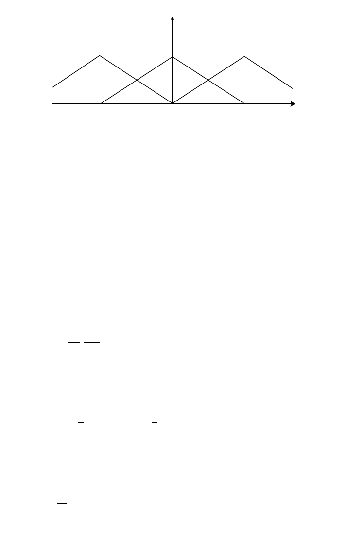
Figure 2.1 Piecewise linear trial functions

where the trial functions w

(x) have the form (see Figure 2.1)

(x) =

⎧

⎪

⎨

⎪

⎩

0, x < x

i−1

x − x

i−1

, x

i−1

≤ x ≤ x

i+1

− x

, x

≤ x ≤ x

i+1

0, x > x

i+1

The expansion coefﬁcient can be found from a system of linear equations obtained

by multiplying the initial equation (2.1) by a verifying function w

(x) and integrating

the resulting equation over the entire domain. In view of the ﬁniteness of the trial

functions, we obtain:



i+1

i−1

k(x)

dx +



i+1

i−1

q(x)y(x)w

(x) dx =



i+1

i−1

f (x)w

(x) dx.

Substitution of (2.22) yields the three-point difference equation (2.20). For A,we

obtain representation (2.16) with a mesh function a

that depends not only on k(x),but

also on q(x):



i−1

k(x) dx −



i−1

q(x)(x − x

i−1

)(x

− x) dx. (2.23)

For smooth coefﬁcients k(x), application of simplest quadrature formulas yields

(2.17).

For the right-hand side and for the coefﬁcient c

in (2.16) we obtain:





i−1

q(x)(x − x

i−1

) dx +



i−1

q(x)(x

i+1

− x) dx



, (2.24)





i−1

f (x)(x − x

i−1

) dx +



i−1

f (x)(x

i+1

− x) dx



. (2.25)

Section 2.1 Finite-difference problem 25

Even in the simplest case of constant coefﬁcients k(x) and q(x), we arrive at an un-

usual approximation of the lowest term in A.

Difference schemes with basis functions chosen in the form of piecewise polyno-

mials of higher degree (quadratic, cubic, etc.) can be constructed in a similar manner.

In the treatment of convection-diffusion problems (see equation (2.5)), FEM schemes

based on the Petrov–Galerkin method have gained acceptance, in which trial and ver-

ifying functions differ from each other. Along this line, in particular, ﬁnite element

analogues of ordinary difference schemes with directed differences can be constructed.

2.1.4 Balance method

Normally, differential equations reﬂect one or another law of conservation for elemen-

tary volumes (integral conservation laws) on contraction of the volumes to zero. In

fact, construction of a discrete problem implies a reverse transition from a differential

to an integral model. One can reasonably demand that, upon such a transition, the con-

servation laws remained fulﬁlled. Difference schemes expressing conservation laws

on a grid are called conservative difference schemes.

Construction of conservative ﬁnite-difference schemes can be reasonably started

from conservation laws (balances) for individual meshes of the difference scheme.

This construction method for conservative difference schemes received the name

integro-interpolation method (balance method). This approach is also known as ﬁnite-

volume method. The integro-interpolation method was proposed by A. N. Tikhonov

and A. A. Samarskii in the early 50ths.

Consider the integro-interpolation method as applied to construction of a difference

scheme for the model one-dimensional problem (2.1), (2.2). Let us consider Q(x) =

−k(x)du/dx. We choose the control volumes as the segments x

i−1/2

≤ x ≤ x

i+1/2

where x

i−1/2

= (i − 1/2)h. Integration of (2.1) over the control volume x

i−1/2

≤ x ≤

i+1/2

yields:

i+1/2

− Q

i−1/2



i+1/2

i−1/2

q(x)u(x) dx =



i+1/2

i−1/2

f (x) dx. (2.26)

The balance relation (2.26) reﬂects a conservation law for the segment x

i−1/2

≤

x ≤ x

i+1/2

. The quantity Q

i±1/2

is the ﬂux through the section x

i±1/2

. Unbalance

between these ﬂuxes is caused by distributed sources (right-hand side of (2.26)) and

by additional sources (integral in the left-hand side of the equation).

To derive a difference equation from the balance relation (2.26), one has to use

some completion of mesh functions. We seek the solution itself at integer nodes (y(x),

x = x

), and ﬂuxes, at half-integer nodes (Q(x), x = x

i+1/2

). We express the ﬂuxes

at half-integer nodes in terms of the values of u(x) at nodal points. To this end, we