Schulz M. Control Theory in Physics and Other Fields of Science: Concepts, Tools, and Applications

Подождите немного. Документ загружается.

4.2 Control by External Sources 105

(r,t)

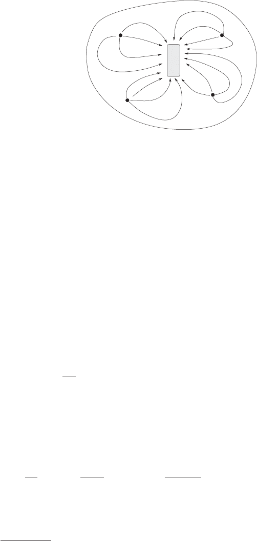
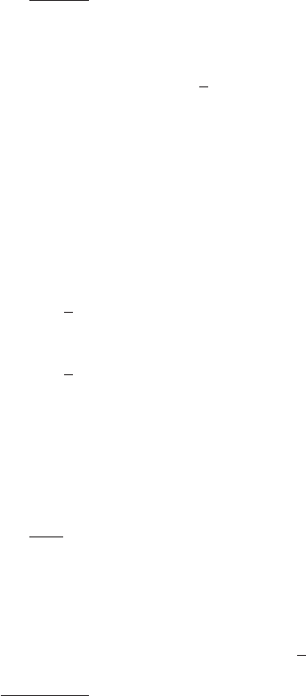
Fig. 4.2. A typical example for a control via external sources: The changes of the

sources u(r, t) propagate due to the ﬁeld Ψ (r, t) in the region under control

R[Ψ,u]=

∞



−∞



rφ(t, r,Ψ(r,t), ∇Ψ (r,t),...,u(r,t), ∇u(r,t),...) .(4.30)

The integration is taken over all points of the d-dimensional space R

and

over all times so that no boundary conditions occur. Therefore, this problem

is called a ﬁeld control problem without boundaries.

As in Sect. 2.4.1, (4.29) and (4.30) can be combined to a common gener-

alized action

S[Ψ, Π,u]=

∞



−∞



rL(t, r,Ψ,Π,u) (4.31)

with the Lagrangian

L = φ(t, r,Ψ,∇Ψ, ∇

Ψ,...,u,∇u, ∇

u, ...)

+Π



∂Ψ

∂t

− F



t, r,Ψ,∇Ψ,∇

Ψ,...,u,∇u, ∇

u,...,J





(4.32)

and the generalized momentum ﬁeld or adjoint ﬁeld Π = Π(r,t). The

derivation of the Euler–Lagrange equations follows the same procedure as

in Sect. 4.1.1. The variation with respect to the generalized momentum ﬁeld

reproduces the ﬁeld equations while the variation with respect to the control

ﬁelds leads to





∂

∂u

−



i=1

∇

∂

∂∇



i,j=1

∇

∂

∂∇

∇

±···





[φ − (Π | F )] = 0 , (4.33)

where we have used, as in Chap. 2.4.1 the vector scalar product (Π | F )in

order to avoid confusions with respect to the presence of more than two vec-

tors

In the present case F , Π,and∂/∂u.

106 4 Control of Fields

The last group of equations is the set of the adjoint evolution equations

following from the variation with respect to Ψ . Here, we obtain

∂Π

∂t





∂

∂Ψ

−



i=1

∇

∂

∂∇



i,j=1

∇

∂

∂∇

∇

±···





× [φ − (Π | F )] (4.34)

with ∇

= ∂/∂r

. The set of equations (4.29), (4.33), and (4.34) is a system of

partial diﬀerential equations solving the optimal control problem

. A general

solution of these more or less formal equations cannot be expected.

From this point of view, a speciﬁcation of the class of ﬁeld theories seems

to be necessary. Fortunately, most of the known and physically realistic ﬁeld

equations are linear expressions in the spatial derivatives

of the ﬁeld func-

tions. Furthermore, these equations contain no derivatives ∇u, ∇

u, ... and

they are only linearly coupled with the control ﬁeld u. In this case, we may

formally rewrite the ﬁeld equations (4.29)as

∂Ψ(r,t)

∂t

FΨ(r,t)+V (r,t,Ψ)

+A(r,t,Ψ)u(r,t)+B (r,t,Ψ) J(r,t) (4.35)

with the N component vector V ,theN ×n matrix A and the N ×n



matrix

B. The linear operator

 is deﬁned by

F =



i=1

(r,t,Ψ) ∇



i,j=1

(r,t,Ψ) ∇

∇

+ ... , (4.36)

and it contains the diﬀerentiable N ×N matrices F

(r,t,Ψ), F

(r,t,Ψ) ,....

The second speciﬁcation belongs to the performance integral. In many appli-

cations it is suﬃcient to assume a performance function of the type

φ = Q (r,t,Ψ)+



α,β=1



i=1

(∇

) Ω

αβ

(r,t)(∇

)+R(r,t,u) (4.37)

with the symmetric matrix Ω of rank N ×N. The component representation is

chosen to obtain a clear representation. The performance (4.37) is suﬃcient for

many problems. The insertion of (4.37) and (4.35)in(4.34) yields the adjoint

ﬁeld equations (now in the component representation with γ =1,...,N)

∂Π

∂t

∂Q

∂Ψ

−



β=1

∇(Ω

γβ

∇Ψ

) −



α=1

∂V

∂Ψ

−



α=1



β=1

∂A

αβ

∂Ψ

In this chapter we refrain from an additional indication of the optimal solution,

i.e., we continuously use Ψ, Π,andu instead of the correct style Ψ

∗

, Π

∗

,andu

∗

The only exception in the above-introduced ﬁeld theories is the equation for the

entropy balance (4.24).

4.2 Control by External Sources 107

−



α=1





β=1

∂B

αβ

∂Ψ

−



α,β=1

αβ

−



α=1

†

γα

(4.38)

with the adjoint operator

†

= −



i=1

∇

(r,t,Ψ)+



i=1

∇

(r,t,Ψ)+··· (4.39)

and the N operators



i=1

∂F

∂Ψ

∇



i,j=1

∂F

∂Ψ

∇

+ ... . (4.40)

Furthermore, the control laws (4.33) are reduced to a simple algebraic law

∂R(u)

∂u



α=1

µα

(r,t,Ψ)Π

(4.41)

with µ =1,...,n.

Example: Economic Field Theories

An interesting, but not directly physically motivating example of ﬁeld control

without boundaries are so-called economic ﬁeld theories [67]. Such theories

have a more or less economic origin. A natural way to handle an economic

system at large scales consists in embedding these into a two-dimensional ge-

ographic space and, subsequently, a continuous description. Such a procedure

reduces the detailed economic relations to several economic and social ﬁelds

satisfying suitable ﬁeld equations. Various publications [68, 69, 70, 71, 72, 78]

deal with such economic ﬁeld theoretical concepts. We remark that other

names, such as urban ﬁelds, continuous ﬂow models, or spatial economy are

also popular.

Historically, the ﬁrst problems of this kind were analyzed by Th¨unen in

1826 [74]. He found that agricultural production would be distributed among

a set of concentric rings around the central town, i.e., a singular consumption

region, according to the cost of transportation. Heavy or bulky goods, such

as wood for energy production and building trade would be produced closer

to the city, while goods more easily transportable farther away. This special

theory is also known as land use model.

Other early publications [75, 76], so-called location theories, consider the

location of production plants instead of consumers. The standard theory of

spatial economics was developed in the early 1950s [70, 77]usingEuler-

Langrange variation principles and hydrodynamic concepts. As such the model

is extremely elegant and versatile, being able to represent all previously known

108 4 Control of Fields

continuous models as special cases. Here, we will give a simple example [78]in

order to demonstrate the basic ideas and the relation to the control of physical

ﬁeld theories.

In a two-dimensional space, the trade ﬂow can be represented by a vector

ﬁeld v(r,t)=(v

(r,t),v

(r,t)) with r =(r

). The absolute value of the

trade ﬂow, |v(r,t)|, represents the quantity of goods traded, whereas the unit

direction ﬁeld n = v/ |v| deﬁnes the local direction of the ﬂow. Just as the ﬂow

of a liquid satisﬁes various balance equations controlling the local conservation

of mass, momentum, or energy, the ﬂow of traded commodities is deﬁned by

a balance equation

∂c(r,t)

∂t

+div v(r,t)=u(r,t) . (4.42)

The source term u(r,t) is related to the local excess supply of production over

consumption and can be interpreted as control ﬁeld. Positive values of u(r,t)

correspond to local sources of commodities due to production centers while

negative values of u(r,t) represent a local excess of consumers. The quantity

c(r,t) deﬁnes the local stock on hand. In general, we can expect that c(r,t)

depends on the local number of traded goods. Hence we get a relation of the

type

c(r,t)=c(|v(r,t)|) . (4.43)

For example, a possible assumption is a power law c = c

|v(r,t)|

with the

reserve exponent β.

In order to determine the trade ﬂow we need a further equation. This

equation follows from the economic principle of minimum transportation costs.

We assume a cost ﬁeld κ(r) which is determined by the local state of the

infrastructure and the structure of the ground. Then, the total transportation

costs K(t) at a given time t are given by [70, 79, 71]

K(t)=



r |v(r,t)|κ(r) , (4.44)

where we have assumed an inﬁnitely large area, and the total transportation

costs over the whole period

are given by



K =

∞



−∞

dtK(t) . (4.45)

Furthermore, the costs also depend on the control ﬁeld u(r,t). We must be

aware that the local excess depends on the geographical landscape. Obviously,

there exist regions which are favored for the settlement of production plants

while other regions are more appropriate for residential areas. Therefore, with-

out any reference to the transportation costs, there exists a natural excess

(r) which is, of course, deﬁned by the landscape. A large positive deviation

We assume here a inﬁnite large period, −∞ <t<∞.

4.2 Control by External Sources 109

u(r,t)− u

(r) means a large local production and consequently a strong con-

tamination of the environment which requires additional high-cost measures

in order to avoid these unwanted side-eﬀects. On the other hand, strongly

negative values of u(r,t) −u

(r) represent a strong density of consumers and

therefore higher costs for the maintenance of buildings and infrastructure.

Thus, we should complete (4.45) by an additional contribution in order to

obtain the performance functional

R =

∞



−∞

dtd



|v(r,t)|κ(r)+

(u(r,t) − u

(r))



. (4.46)

These relation and the ﬁeld equation (4.42) build the complete ﬁeld control

problem. First of all, we extract the Lagrangian

L = |v(x,t)|κ(r)+

(u(r,t) − u

(r))

+ Π(r,t)



∂c(|v(r,t)|)

∂t

+div v(r,t) − u(r,t)



. (4.47)

This representation requires two important remarks. First of all, we must

consider that (4.42) is a one-component ﬁeld equation. That means only one

degree of freedom of the vector v =(v

) can be interpreted as a state

ﬁeld in the sense of the control theory, the other degree of freedom is simply

another control ﬁeld. Therefore, the generalized momentum Π(r,t)isonlya

scalar ﬁeld. The second remark concerns the ﬁeld equation itself. Obviously,

(4.42) is a ﬁeld equation in an implicit representation. However, the structure

of (4.47) may be changed by an appropriate transformation of the general-

ized momentum in such a manner that the last contribution contains a ﬁeld

equation in the explicit form.

The variation of the action corresponding to (4.47) with respect to the con-

trol ﬁeld, the state ﬁeld, and the momentum ﬁeld yields the Euler–Lagrange

equations. Especially, the variation with respect to v(r,t) leads to



κ(r) − c



(|v(r,t)|)

∂Π(r,t)

∂t



v(r,t)

|v(r,t)|

= ∇Π(r,t) . (4.48)

The compact form of (4.48) partially hides the fact that these equations are

essentially one equation for the state ﬁeld and one for the second control ﬁeld.

The variation with respect to Π(r,t) leads again to (4.42), while the variation

with respect to the ﬁrst control ﬁeld gives

u(r,t) − u

(r)=Π(r,t) . (4.49)

Equations (4.42), (4.48), and (4.49) form a complete ﬁeld-theoretical problem.

Unfortunately, these equations are dominated by strong nonlinearities. This

problem also remains if we focus in particular on the steady state. This special

case reduces the ﬁeld equations to

110 4 Control of Fields

κ(r)

v(r)

|v(r)|

= ∇Π(r) and div v(r)=Π(r)+u

(r) . (4.50)

The decomposition of the transport ﬁeld v(r) into a vortex-free part ∇ϕ and

a divergent-free part w(r) with div w(r) = 0 transforms the second equation

into the two-dimensional Poisson equation

∇

ϕ(r)=Π(r)+u

(r) . (4.51)

The solution of this equation is possible with well-known standard methods if

Π(r) is known. The second step is the determination of the scalar momentum

ﬁeld Π(x). If we take squares of both sides of the ﬁrst equation of (4.50), we

obtain the closed nonlinear ﬁeld equation

(∇Π)



∂Π

∂r





∂Π

∂r



= κ(r) . (4.52)

The local transportation costs κ(r) are, just as the quantity u

(r), an external

ﬁeld which may be empirically determined by suitable observations or estima-

tions. Finally, inserting the solution of (4.52) into the ﬁrst equation of (4.50)

we obtain a nonlinear, algebraic equation for the ﬁeld w(r) which depends on

the local structure of the ﬁelds ϕ(x)andΠ(r).

The present theory allows the construction of optimal roads. Let us assume

that we know the scalar ﬁeld of the transportation costs κ(r). As discussed

above, the vector ﬁeld v(r) deﬁnes the direction of the local ﬂow. A road may

be deﬁned by the curve y(s) where s is an arbitrary curve parameter. Then

the tangent of an optimal road

t (s)=

dy (s)

(4.53)

always shows in the direction of the local ﬂow. That means we have the relation

t (s)=

v(y (s))

|v(y (s))|

(4.54)

along the road. Therefore, we expect that an optimal road fulﬁls the equation

κ(y (s))t (s)=κ(y (s))

v(y (s))

|v(y (s))|

= ∇Π(y (s)) . (4.55)

Let us try to eliminate the momentum ﬁeld Π from (4.55). To this aim we

diﬀerentiate with respect to the curve parameter



κ(y (s))

dy (s)



∇Π(y (s)) . (4.56)

The vector components on the right-hand side can be written as

∂Π(r)

∂r



r=y(s)



j=1

∂

Π(r)

∂r



r=y(s)

∂y

(s)

∂s



j=1

∂

Π(r)

∂r



r=y(s)

(s) . (4.57)

4.2 Control by External Sources 111

We multiply this expression with κ(y (s)) and apply (4.55) in order to obtain

κ(y (s))

∂Π(r)

∂r



r=y(s)



j=1

∂

Π(r)

∂r



r=y(s)

∂Π(r)

∂r



r=y(s)

(4.58)

∂

∂r



j=1



∂Π(r)

∂r





r=y(s)

(4.59)

or with (4.52)

κ(y (s))

∇Π(y (s)) =

∇κ(r)|

r=y(s)

. (4.60)

Considering (4.55), we obtain the optimal road equation

κ(y (s))



κ(y (s))

dy (s)



∇κ(y (s)) . (4.61)

We remark that the last equations are close to Fermat’s law in optics. In

particular, roads are equivalent to light rays, the momentum ﬁeld corresponds

to the eikonal function, and the transportation cost may be interpreted as

the refraction index. For example, if we have spatially separated types of

transportation, for example transportation over sea and over land, the trading

routes are straight lines, broken at the coastline via the well-known refraction

law [80, 81]. A similar phenomenon belongs to roads through high mountain

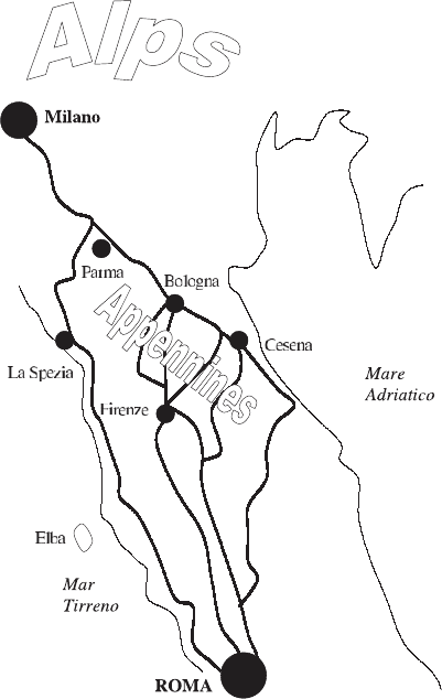
regions. For instance, the highways from Rome to Milan pass the Appenines

in a similar way as light rays pass a glassy plate; see Fig. 4.3.

Pontryagin’s Maximum Principle

If the Lagrangian depends only on the control ﬁeld u but not on the spatial

derivatives ∇u, ∇

u,..., we are able to apply Pontryagin’s maximum prin-

ciple. In other words, we search for the control ﬁeld u(r,t) which minimizes

the Lagrangian (4.32) at each point (r,t) and for each ﬁeld conﬁguration



Π, Ψ, ∇Ψ,∇

Ψ, ...



. As in the case of systems with a ﬁnite degree of freedom,

we may deﬁne the preoptimized ﬁeld, u

(∗)



r,t,Π,Ψ,∇Ψ,∇

Ψ, ...



, which sat-

isﬁes the inequality



t, r,Π,Ψ,∇Ψ,∇

Ψ,...,u

(∗)

(t, r,Π,Ψ,∇Ψ,∇

Ψ,...)



≤L



t, r,Π,Ψ,∇Ψ,∇

Ψ,...,u



(4.62)

for all allowed control ﬁelds u. The Pontryagin maximum principle allows the

extension of the ﬁeld control problem to control ﬁelds u (t, r) restricted to

an arbitrary, possibly time- and space-dependent region U



(r,t)⊂ U. In other

words, the preoptimized Lagrangian is then given by

112 4 Control of Fields

Fig. 4.3. Schematic representation of the highways from Rome to Milan

(∗)



t, r,Π,Ψ,∇Ψ,∇

Ψ,...



= L



t, r,Π,Ψ,∇Ψ,∇

Ψ,...,u

(∗)

(t, r,Π,Ψ,∇Ψ,∇

Ψ,...)



= min

u∈U



(r,t)⊂U



t, r,Π,Ψ,∇Ψ,∇

Ψ,...,u



. (4.63)

The Pontryagin maximum principle becomes important if the control law,

∂L/∂u = 0, see for example (4.41), as a specialized version has no global

minimum solution inside the allowed set U



(r,t).

Linear–Quadratic Problems

The system of partial diﬀerential equations consisting of the ﬁeld equations

(4.35), the adjoint ﬁeld equations (4.38), and the control law (4.41) is again

4.2 Control by External Sources 113

a strongly nonlinear problem. Most of such problems

have to be solved

numerically and it is often uncertain whether the applied numerical algorithm

has actually found the correct solution.

However, a systematic procedure is possible for linear–quadratic problems.

To this aim we consider linear ﬁeld equations. This may be physically moti-

vated by the circumstance that a large class of classical ﬁeld theories automat-

ically generates linear ﬁeld equations because linearity is a necessary condition

for ﬁelds satisfying the superposition principle. Linear ﬁeld equations are a

special class of (4.35) and may be written in the form

∂Ψ(r,t)

∂t

FΨ(r,t)+Au(r,t)+BJ(r,t) (4.64)

with the matrices A = A(r,t)andB = B(r,t) and the linear operator

F = F



i=1

∇



i,j=1

∇

+ ... (4.65)

with the matrices F

(r,t), F

(r,t), .... We remark that without any

restrictions the matrix B can be combined with the external sources J to a

common quantity, BJ → J. This is not generally allowed for the matrix A and

the control ﬁelds u. If we replace Au → u we must simultaneously substitute

u → A

−1

u in the performance functional. But this is possible only if the

inverse matrix A

−1

exists for all points (r,t) of the space–time continuum.

Furthermore, the performance may be characterized by the quadratic form

φ =



α,β=1



αβ

(r,t) Ψ



i=1

(∇

) Ω

αβ

(r,t)(∇

)





α,β=1

αβ

(r,t) u

(4.66)

which is a specialized version of (4.37). The symmetric matrix Q is of order

N × N , while the symmetric matrix R has the rank n × n. Considering the

above-introduced linear structure of the ﬁeld equations and the quadratic form

of the performance, we obtain the adjoint ﬁeld equations

∂Π

∂t



β=1

γβ

(r,t) Ψ

−∇(Ω

γβ

∇Ψ

)] −



α=1

†

γα

, (4.67)

which depend no longer on the control ﬁelds and other external sources. The

adjoint operator F

†

is deﬁned by

†

= F

(r,t) −



i=1

∇

(r,t)+



i,j=1

∇

(r,t)+··· . (4.68)

The control of hydrodynamic equations yields several standard examples for such

a nonlinear coupled system of partial diﬀerential equations.

114 4 Control of Fields

Thus, the adjoint ﬁeld equation is also linear. Finally, we get the linear control

law



α=1

γα

(r,t) u



α=1

µα

(r,t)Π

. (4.69)

If R

−1

exists, (4.69) may be used for the elimination of the control ﬁelds

from the ﬁeld equations (4.64). Thus, the linear–quadratic control problem

leads to a system of 2N coupled linear partial diﬀerential equations for the N

components of the ﬁeld Ψ and the N components of the momentum ﬁeld Π.

Such systems can be solved by various approximative numerical techniques.

A standard method is the expansion of the pair of ﬁeld components in terms

of a complete set of orthogonal functions or basic functions. This reduces the

system of partial diﬀerential equations to an inﬁnitely large linear algebraic

system. Such a system can be solved numerically if only a ﬁnite subset of

orthogonal functions is taken into account. In principel, this approximative

solution should converge to the true solution with an increasing number of

considered basic functions. The convergence velocity depends strongly on the

type of the more or less empirically chosen set of orthogonal functions. The

choice of an appropriate set of basic functions is often a question of the nu-

merical and scientiﬁc experience with respect to the underlying problem.

4.2.3 Passive Boundary Conditions

Passive boundary conditions occur if we have a ﬁeld under control in a certain

spatial region with unchangeable boundary conditions. In other words, the

boundaries cannot be used for a control of the ﬁelds. The above-introduced

techniques can also be extended to those boundary problems. However, just as

in the case of optimal ﬁeld control without boundaries, it remains the general

situation that systematic concepts for solving such problems exist only for

linear ﬁeld equations. A very elegant method is the application of Green’s

functions. The knowledge of these functions allows the solution of linear ﬁeld

equation for arbitrary sources, but with well-deﬁned boundary conditions.

Let us assume that the linear equation (4.64) is declared over a well-deﬁned

region G of the space R

and that the ﬁeld has at the border ∂G well-deﬁned

boundary conditions. Then, the formal solution of (4.64) is given by

Ψ (r,t)=Ψ

hom

(r,t)+



dτ



xΓ (r,t| x,τ)[Au(r,τ)+BJ(r,τ)] (4.70)

with the so-called Green function Γ (r,t | x,τ) and the homogeneous solution

hom

(r,t) satisfying

∂Ψ

hom

(r,t)

∂t

FΨ

hom

(r,t) . (4.71)