Sha W., Malinov S. Titanium Alloys: Modelling of Microstructure, Properties and Applications

Подождите немного. Документ загружается.

Titanium alloys: modelling of microstructure208

(i) The creation of a volume V of α phase will cause a free energy reduction

of V∆g where ∆g is the free volume energy of nucleation or driving

force;

(ii) The creation of area S of interface will give a free energy increase of

Sγ;

(iii) The transformed volume will not fit perfectly into the space originally

occupied by the matrix and this gives rise to a misfit strain energy ∆G

per unit volume of α.

Summing all of these gives the total free energy change as

∆G* = –V∆g + Sγ + V∆G

[8.1]

The nucleus of the α phase forms preferentially at a β grain boundary because

the interfacial energy term will be reduced and some free energy will be

released, thereby reducing the activation energy barrier. Ignoring any misfit

strain energy, the optimum embryo shape should be that which minimises

the total interfacial free energy – two abutted spherical caps with wetting

angle θ given by

cos =

ββ

αβ

[8.2]

The excess free energy associated with the embryo will be given by

∆G* = –V∆g + S

αβ

– S

ββ

[8.3]

where V is the volume of the embryo, S

αβ

is the area of α/β interface of free

interface energy γ

αβ

created, and S

ββ

the area of β/β grain boundary of

energy γ

ββ

destroyed during the process.

The above equation can be written in terms of the wetting angle θ and the

cap radius r as

∆∆GrgrS* = –

+ 4 ( )

ππγ

αβ

()

[8.4]

where S(θ) is a shape factor given by

S () =

(2 + cos )(1 – cos )

θθθ

[8.5]

By differentiation of Eq. [8.4], it can be shown that the critical radius for

nucleation is

2γ

αβ

∆

[8.6]

and the activation barrier for nucleation is

∆

()

πγ

αβ

[8.7]



Finite element method: morphology 209

The nucleation rate is given by an equation of the form

exp –

∆





















[8.8]

where N

is the number of nucleation sites (atoms) per unit volume, ∆G

, the

activation energy for atomic migration across the interface, k

, the Boltzmann

constant, T, the temperature in Kelvin, and h, the Planck constant.

can be assumed to be constant. ∆G

is usually assumed to be half of

the activation energy for diffusion (Wilkinson, 2000). Note that the diffusion

of vanadium away from the interface is considered in the growth theory

further below, where the activation energy for bulk diffusion is used.

∆G

strongly depends on the temperature and the concentration of vanadium in

the β phase. The interface energy γ

αβ

can be considered as temperature and

vanadium concentration independent and is a free parameter in the model,

which is obtained by fitting the calculated results to the microstructural

observations.

At each time-step, we calculate the number of nuclei on the grain boundary

area S

occupied by the β-phase using

exp –

∫∫





















∆

[8.9]

At the moment that the number of nuclei increases by one, a new nucleus is

generated on the β phase surface. The probability for a nucleus to appear at

a point x of the grain boundary area S

, occupied by the β phase, is proportional

to the exponent of the activation energy and depends on the temperature and

vanadium (the alloying element to be redistributed) concentration C:

Px P

GTCx

( ) = exp –

(, ())

∆













[8.10]

The coefficient P

is determined from the requirement that the total probability

for a new nucleus occurring on the grain boundary area S

at the moment t

is equal to 1:

1 = exp –

(, ())

GTCx

∫













∆

[8.11]

8.4.2 Growth of α phase lamellae

The evaluation of aluminium and vanadium contents in the α and the β

phases indicates that the migration of the interface is controlled mainly by

the transfer of vanadium atoms (Fig. 5.1 and Chapter 6). For simplicity, we



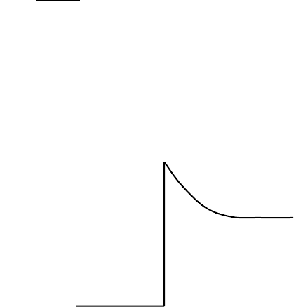
Titanium alloys: modelling of microstructure210

consider the migration of the interface separating the two phases as a result

of the flux of vanadium atoms from α to β phase. As the precipitate grows,

the α becomes depleted of vanadium so that the β vanadium concentration

adjacent to the interface C

increases above the initial vanadium concentration

in the β phase C

(see Fig. 8.3).

The rate at which an interface moves depends both upon intrinsic mobility,

which is related to the process of vanadium atom transfer across the interface,

and on the rate at which lattice diffusion can remove the excess of vanadium

atoms ahead of the interface. If the interfacial reaction is fast, i.e. the transfer

of atoms through the interface is an easy process, the growth is known as

diffusion controlled. However, if, for some reasons, the interfacial reaction

is much slower than the rate of diffusion, the growth rate will be governed

by interface kinetics. The growth is said to be interface controlled.

The two processes are in series so that the interface flux calculated from

the interface mobility always equals the flux calculated from the diffusion

ahead of the interface.

Since the growth of the precipitate requires a flux of vanadium atoms

from α to β phase, there must be a positive driving force across the interface

− difference in the chemical potential that drives the vanadium atoms across

the boundary ∆

. Clearly, for growth to occur, the interface composition C

must be lower than the equilibrium vanadium concentration in the β phase

. The corresponding flux across the interface will be given by

∆

[8.12]

where M is the interface mobility and V

is the molar volume of the α

phase.

α phase β phase

8.3

Vanadium concentration profile at the α/β interface.



Finite element method: morphology 211

As a result of the concentration gradient in the β phase, there will also be

a flux of vanadium atoms removing the excess of vanadium ahead of the

interface given by

JDC

interface

∇|

[8.13]

where D is the diffusion coefficient of vanadium. If a steady state exists at

the interface, these two fluxes must balance:

[8.14]

The diffusion process and the concentration of vanadium in the β phase can

be calculated by solving the classical diffusion equation in appropriate initial

and boundary conditions:

∂

∇⋅ ∇

DC = ( )

[8.15]

Ignoring the heat absorbed or evolved and volume changes during the process

of phase transformation, the free energy change is due only to the change in

entropy. In this case the driving force ∆

is given as

∆

( – )

[8.16]

Then, the boundary condition Eq. [8.12] can be written in the form

int

( – )

[8.17]

The α/β interface is not stationary but moves as diffusion progresses. If a

unit area of the α/β interface advances a small distance dx, a volume dx · 1

will be converted from α containing C

amount of vanadium to α containing

, where C

and C

are the concentrations of vanadium at the interface in α

and β phases, respectively. This means that the amount of vanadium removed

from α phase and partitioned into β is given by

– C

) dx [8.18]

In order to maintain the mass balance at the interface, this amount of vanadium

must equal the product

( ) d

⋅⋅n

, where

⋅ n

is the flux of vanadium

atoms diffusing away from the interface in a direction n normal to the interface

(Borgenstam et al., 2000). Therefore,

– C

)dx = D(n · ∇C)|

int

dt [8.19]

The growth rate is then given by

(– )

( )

int

n ⋅∇ |

[8.20]



Titanium alloys: modelling of microstructure212

If the interface mobility M is very high, ∆

can be very small and

≈

Under these circumstances, there is effectively local equilibrium at the interface.

The interface will then move as fast as diffusion allows, and growth will take

place under diffusion control. The growth rate then can be evaluated as a

function of time t by solving the diffusion equation in the area occupied by

the β phase with the boundary condition at the α/β interface given by

[8.21]

When the interface has a lower mobility, a greater chemical potential difference

∆

is required to drive the interface reaction and there will be a departure

from the local equilibrium at the interface. The value of C

will be that which

satisfies the flux balance equation Eq. [8.14]. The growth rate then can be

evaluated by solving the diffusion equation in the area occupied by the β

phase with the boundary condition at the α/β interface given by Eq. [8.17].

8.4.3 Localisation of the α/β interface

The most important task in the analysis of the β to α transformation is the

determination of the location of the moving α/β interfaces for all of the

Widmanstätten α plates. Methods employed to solve such a problem can be

classified into two groups: Lagrangian and Eulerian schemes. The Lagrangian

scheme is characterised by the mesh which is moved or deformed with the

progress of the calculation. The mesh boundaries coincide with the free

surface. However, over-distorted meshes due to the growth of the great number

of Widmanstätten α plates in different directions may result in numerical

errors. In Eulerian schemes, computational meshes are generated beforehand

and fixed during the entire calculation. Therefore, they are free from the

difficulties due to the deforming of meshes. However, a special treatment is

necessary to track the moving free surface. The volume of fluid (VOF)

method, introduced by Hirt and Nichols, is popular in flow problems with

moving free surface. In this method, the entire domain is divided into cells

and the volume fraction of fluid in each cell is defined. The flow front is

advanced by solving the following transport equation:

∂

∇⋅

F + ( ) = 0v

[8.22]

Here F is the volume fraction of the fluid in a cell and v is the flow velocity

vector.

A computer code based on the finite element method and the VOF method

is developed to trace the moving α/β interface. Instead of fluid, we consider

the volume fraction F of the α phase in the finite elements. Depending on the

value of the α phase volume fraction F in an element, the entire domain is

divided into three categories by the following criterion:



Finite element method: morphology 213

Fxt(, ) =

volume of phase

volume of element

1 filled

> 0 and < 1 partially filled

0 empty











[8.23]

F is unity in the α phase regions and zero in the β phase region. Therefore,

the α/β interface can be considered to exist in the partially filled elements

with F values between 0 and 1. In order to represent the interfaces, it is

convenient to use nodal values. A control volume is associated with each

nodal point and the α phase fraction of a nodal control volume is taken as the

average of the α-phase fractions of the elements surrounding the corresponding

node

[8.24]

where superscript i denotes the ith nodal point, and subscript k indicates a

surrounding element.

is the volume of the corresponding element, and

is its α phase fraction. The shape of the α/β interface is represented by

contour lines connecting nodal points along which the volume fractions are

such that

0.5 < 1

≤ F

In order to locate the interface precisely, the number of partially filled

elements should be kept as small as possible. However, as Eq. [8.22] is

solved numerically, the interface region becomes wider as time progresses

due to false numerical diffusion of F. The donor-acceptor scheme is a popular

method for overcoming such smearing of the free surface. Instead of solving

Eq. [8.22] directly, volume flux across the element boundary is estimated

and the change in F of the element is monitored.

For the location of the α/β interface, we integrate the equation of the α

phase volume fraction Eq. [8.22] only for partially filled elements.

Discretisation by the explicit scheme gives

new old

= + – ( )d

∆

∫

⋅













[8.25]

where

new

and

old

are the volume fractions of α phase in element k at

previous and present times, ∆t is the calculation time step, v is the growth

rate and S

is the boundary of the element. The last term in Eq. [8.25]

represents the increase of F due to the incoming flux of vanadium atoms

across the α/β interface. F

is the value of F on the boundary, defined as

phase volume transfered through

total value transfered through

[8.26]

where l denotes the l th boundary of the k th element. Once F

is known, the



Titanium alloys: modelling of microstructure214

integral in Eq. [8.25] can be evaluated to give the net flux of F into the

element i. F values after time interval ∆t can then be updated and the α/β

interface location can be determined. Therefore, the problem is simplified

down to the determination of the value of F

. We use an algorithm proposed

by Shin and Lee (2000) to determine the α phase flux across the boundary

. The proposed scheme uses the concept of the donor–acceptor method

and is modified to make compatible with FEM.

8.4.4 FEM formulation of the diffusion problem

The finite element method is used for solving the diffusion equation on the

domain occupied by β phase. The elements chosen have dimensions in both

space and time, which allows for the easy determination of the position of

the free surface and also incorporate the natural boundary conditions in a

straightforward manner. The method is essentially an implicit time stepping

technique and therefore is stable even for relatively large time steps.

The finite element approximation is based on the weak form of the diffusion

equation [8.15], which may be written as

∫

∂













– d d = 0

[8.27]

where V is the space–time domain for t > 0

V = {(x

, t): x

∈ V

, t > 0}

is the volume occupied by β phase. The function

is required to be

measurable in the Sobolev sense.

From a computational viewpoint, a more useful weak form is the Galerkin

form, which is derived from Eq. [8.27] by the use of Stock’s theorem. This

form requires minimum continuity of the solutions for C.

vt D

nst

∫∫ ∫

∂

d d + d d – d d = 0

[8.28]

where the integration in s is over the boundary δV

of V

and E is the domain

E = {(x, t): x ∈ δV

, t > 0} [8.29]

The boundary conditions on the α/β interface are incorporated by the

replacement of the flux

∂

of vanadium atoms diffusing away from

the interface in a direction n normal to it with the corresponding flux across

the interface

int

( – )

. Then, Eq. [8.28] is written in the form



Finite element method: morphology 215

vt D

CCst

∫∫ ∫

∂

d d + d d +

( – )dd = 0

[8.30]

Let us assume that the solution of the Eq. [8.30] is given at time t and the

solution at some later time is desired. V

is defined as a region in the space–

time containing the β phase domain between the times t

and t

n+1

= {(x

, t): x

∈ V

, t

≤ t ≤ t

n+1

} [8.31]

Then, Eq. [8.30] may be rewritten as

nn n

vt D

CCst

∫∫ ∫

∂

dd+ dd+

(–)dd=0

[8.32]

where

= {(x

, t): x

∈ δV

, t

≤ t ≤ t

n+1

} [8.33]

We approximate the region V

by a set of finite elements, in particular a set

of four node elements in the two-dimensional case, and introduce parametric

approximations, which map these elements onto a standard square. Clearly,

the elements approximating the regions V

are the quadrilateral bases of the

prisms that approximate the region V

. The subdivision of the domain V

into a set of finite elements reduces the original problem to one which is

finite dimensional and the values of the concentration are calculated only at

the nodes of the elements. In terms of basic function expansion, the

concentration field is taken to be of the form

CC xyCt

= ( , ) ( )

≅

[8.34]

where N is the number of FE mesh nodes, and

ttCttCttt

n+1

() =

(– )

[( – ) + ( – ) ];

+1 +1

≤≤

[8.35]

where

are the nodal values of C at time t

;

are the basic functions,

which are assumed to form a complete set of functions over the β phase

domain volume. The interpolating functions

must be chosen to preserve

continuity of concentration between the elements because of the first order

derivatives in Eq. [8.32]. Here,

are chosen to be a set of bilinear pyramid

functions:

( ) = =

1 =

≠







[8.36]



Titanium alloys: modelling of microstructure216

The Galerkin approximation satisfies

vt D

∫∫

∂

˜˜

dd + dd

( – )dd = 0

CCst

∫

[8.37]

The derivatives of

are calculated in the form

∂

(– )

( – )

[8.38a]

∂

ttCttC

(– )

[( – ) + ( – ) ]

[8.38b]

Substituting the derivatives [8.38] into Eq. [8.37], we obtain a system of

linear equations:

(– )

( – ) d

CC v

∫

φφ

( + ) d

∫

∂

φφ

–

( + ) d +

d = 0

CC s

ββ

∫∫

φφ φ

[8.39]

which can be solved for the unknown nodal values

n+1

of the concentration

field.

The overall numerical procedure is summarised as follows:

(i) Divide the entire domain into meshes.

(ii) Solve the diffusion equation of vanadium in β phase domain by FEM.

(iii) Determine the growth rate of the α/β interface by solving Eq. [8.20].

(iv) Determine the value of F

at each boundary of the partially filled

element.

(v) Calculate the α phase flux into the element.

(vi) Determine the α phase fraction at the new time.

(vii) Define the β phase domain using the updated α phase volume fraction

of the elements.

(viii) Repeat steps (ii) through (vii) until the final temperature is reached.

In summary, the following main assumptions are accepted in the model:

(i) The β to α phase transformation in the Ti-6Al-4V alloy is diffusional.

This assumption is reasonable for the cooling rates (from 5 to 50 °C/min)



Finite element method: morphology 217

and the temperature intervals (from 750 to 1000 °C) applied. However,

this also means that the model simulations cannot be used for higher

cooling rates when a martensitic transformation is involved.

(ii) The diffusional β to α phase transformation at cooling is mainly

controlled by the diffusional redistribution of vanadium between the

α and the β phases toward enrichment of vanadium in the β phase.

This assumption is based on the following.

(a) Thermodynamic calculations performed using the titanium database

show that the major difference in the compositions of the α and

the β phases at different temperatures is their vanadium contents

while the aluminium contents in the two phases are similar (see

Fig. 5.1b).

(b) The diffusion coefficient of vanadium in the titanium matrix is 2

to 3 times lower than that of aluminium in the temperature range.

It is possible to incorporate into the model simultaneous aluminium

redistribution. This, however, would increase significantly the

requirements for computational resources without worthy improvement

of the model simulations.

(iii) The diffusion coefficient, used for the calculation of the vanadium

concentration in the β phase, depends on the temperature by an

Arrhenius-type equation:

= exp –









[8.40]

where A = 1.6 × 10

–4

/s and the activation energy Q =

123.9 kJ/mol.

(iv) In our case we use a value of 62 kJ/mole for ∆G

which is half of the

activation energy for diffusion of vanadium in the β phase.

In the following sections, some of the simulations from the model will be

discussed.

8.5 The 1-D model

The first step is to develop a 1-D model for the β to α phase transformation

in the Ti-6Al-4V alloy. The 1-D model can be used for a description of the

nucleation and growth of the α phase at the grain boundary and for prediction

of the thickness distribution of a group of Widmanstätten plates growing in

parallel direction. We will now simulate the processes of nucleation and

growth for different cooling rates.

Using Thermo-Calc and the titanium database, we calculate the volume

driving force for formation of the α phase for a wide range of temperatures

