Stewart J. Calculus

Подождите немного. Документ загружается.

Then use these sketches to ﬁnd the following limits.

(a) (b)

Find if

for all .

60. (a) A tank contains 5000 L of pure water. Brine that contains

30 g of salt per liter of water is pumped into the tank at a

rate of 25 L#min. Show that the concentration of salt after

minutes (in grams per liter) is

(b) What happens to the concentration as ?

;

61. Use a graph to ﬁnd a number such that

;

62. For the limit

illustrate Deﬁnition 5 by ﬁnding values of that correspond

to and .

;

63. For the limit

illustrate Deﬁnition 6 by ﬁnding values of that correspond

to and .

;

64. For the limit

illustrate Deﬁnition 7 by ﬁnding a value of that corres-

ponds to .

(a) How large do we have to take so that ?

(b) Taking in Theorem 4, we have the statement

Prove this directly using Deﬁnition 5.

lim

x l $

! 0

r ! 2

1#x

0.0001

65.

M ! 100

lim

x l $

2x ! 1

x ! 1

! $

& ! 0.1& ! 0.5

lim

x l "$

! 1

x ! 1

! "2

& ! 0.1& ! 0.5

lim

x l $

! 1

x ! 1

! 2

(

! 1

! x ! 1

" 1.5

(

0.05thenx % N

t l $

C&t' !

30t

200 ! t

x % 5

4x " 1

f &x'

! 3x

lim

f &x'

59.

lim

49.

50.

51–54 Sketch the graph of a function that satisﬁes all of the

given conditions.

, , ,

if , if ,

if or if ,

if , ,

for all

52. , , if ,

if ,

if , ,

for all

53. , , ,

, , ,

for , for and for

54. , for , ,

, ,

55. (a) Use the Squeeze Theorem to evaluate .

;

(b) Graph . How many times does the graph

cross the asymptote?

;

56. By the end behavior of a function we mean the behavior of

its values as and as .

(a) Describe and compare the end behavior of the functions

by graphing both functions in the viewing rectangles

by and by .

(b) Two functions are said to have the same end behavior if

their ratio approaches 1 as . Show that P and Q

have the same end behavior.

Let and be polynomials. Find

if the degree of is (a) less than the degree of and

(b) greater than the degree of .

58. Make a rough sketch of the curve ( an integer)

for the following ﬁve cases:

(i) (ii) , odd

(iii) , even (iv) , odd

(v) , evennn

0nn % 0

nn % 0n ! 0

ny ! x

lim

x l $

P&x'

Q&x'

57.

x l $

*"10,000, 10,000+*"10, 10+*"2, 2+*"2, 2+

Q&x' ! 3x

P&x' ! 3x

" 5x

! 2x

x l "$x l $

f &x' ! &sin x'#x

lim

sin x

lim

x l 0

t)&x' ! $

lim

x l 0

t)&x' ! "$lim

x l $

t&x' ! "$

lim

x l "$

t&x' ! $x " 0t*&x'

0t&0' ! 0

0f *&x'

0x % 2f *&x' % 0

lim

x l $

f &x' ! 0lim

x l "$

f &x' ! $lim

x l 0

f &x' ! "$

lim

x l 2

f &x' ! "$lim

x l 2

f &x' ! $f &1' ! f )&1' ! 0

xf &"x' ! "f &x'

lim

x l $

f &x' ! 0x % 4f *&x' % 0

4f *&x'

0x % 2f )&x'

2f )&x' % 0f )&0' ! 1f )&2' ! 0

xf &"x' ! f &x'

lim

x l $

f &x' ! 11

4f *&x' % 0

x % 40 ( x

1f *&x'

x % 2f )&x' % 00

2f )&x'

f &0' ! 0f &2' ! "1f )&2' ! 0

51.

y ! x

" 1'

&x ! 2'

y ! &3 " x'&1 ! x'

&1 " x'

242

|| ||

CHAPTER 4 APPLICATIONS OF DIFFERENTIATION

SECTION 4.5 SUMMARY OF CURVE SKETCHING

|| ||

243

69. Prove that

and

if these limits exist.

70. Formulate a precise deﬁnition of

Then use your deﬁnition to prove that

lim

x l "$

&1 ! x

' ! "$

lim

x l "$

f &x' ! "$

lim

f &x' ! lim

f &1#t'

lim

f &x' ! lim

f &1#t'

66. (a) How large do we have to take so that ?

(b) Taking in Theorem 4, we have the statement

Prove this directly using Deﬁnition 5.

67. Use Deﬁnition 6 to prove that .

68. Prove, using Deﬁnition 7, that .lim

! $

lim

x l "$

! 0

lim

x l $

! 0

r !

0.0001x

SUM MARY OF CURVE SKE TCHI NG

So far we have been concerned with some particular aspects of curve sketching: domain,

range, and symmetry in Chapter 1; limits, continuity, and vertical asymptotes in Chapter 2;

derivatives and tangents in Chapter 3; and extreme values, intervals of increase and

decrease, concavity, points of inﬂection, and horizontal asymptotes in this chapter. It is

now time to put all of this information together to sketch graphs that reveal the important

features of functions.

You might ask: Why don’t we just use a graphing calculator or computer to graph a

curve? Why do we need to use calculus?

It’s true that modern technology is capable of producing very accurate graphs. But even

the best graphing devices have to be used intelligently. We saw in Section 1.4 that it is

extremely important to choose an appropriate viewing rectangle to avoid getting a mis-

leading graph. (See especially Examples 1, 3, 4, and 5 in that section.) The use of calculus

enables us to discover the most interesting aspects of graphs and in many cases to calcu-

late maximum and minimum points and inﬂection points exactly instead of approximately.

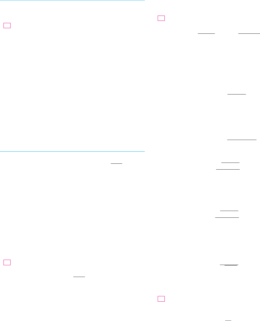
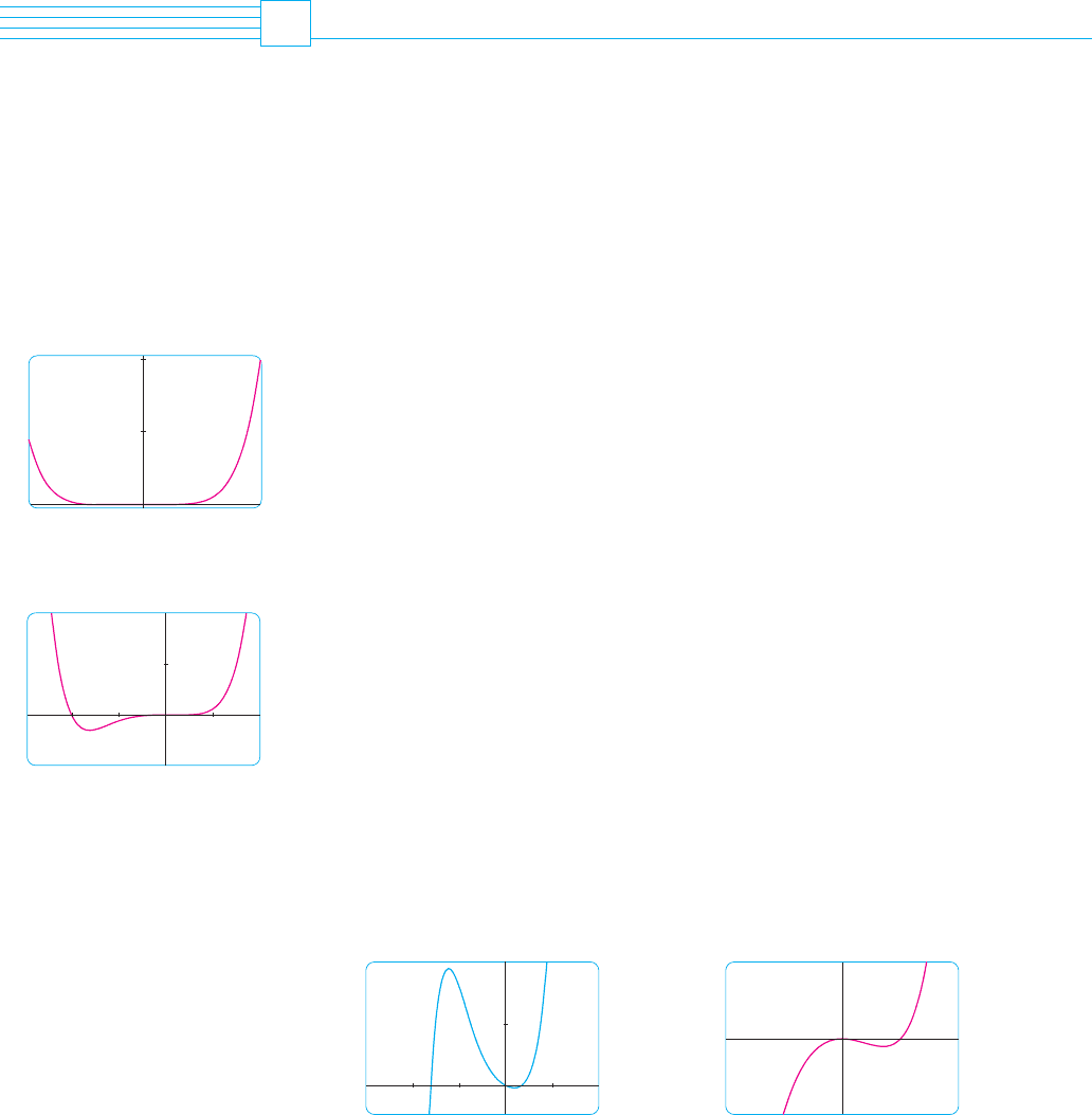
For instance, Figure 1 shows the graph of . At ﬁrst

glance it seems reasonable: It has the same shape as cubic curves like , and it

appears to have no maximum or minimum point. But if you compute the derivative, you

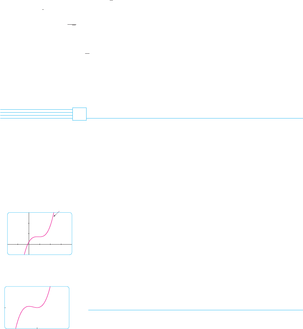
will see that there is a maximum when and a minimum when . Indeed, if

we zoom in to this portion of the graph, we see that behavior exhibited in Figure 2. Without

calculus, we could easily have overlooked it.

In the next section we will graph functions by using the interaction between calculus

and graphing devices. In this section we draw graphs by ﬁrst considering the following

information. We don’t assume that you have a graphing device, but if you do have one you

should use it as a check on your work.

GUIDELIN E S FO R SKE T C H I N G A C U RV E

The following checklist is intended as a guide to sketching a curve by hand. Not

every item is relevant to every function. (For instance, a given curve might not have an

asymptote or possess symmetry.) But the guidelines provide all the information you need

to make a sketch that displays the most important aspects of the function.

A. Domain It’s often useful to start by determining the domain of , that is, the set of

values of for which is deﬁned.f &x'x

y ! f &x'

x ! 1x ! 0.75

y ! x

f &x' ! 8x

" 21x

! 18x ! 2

4. 5

F I G U R E 1

_10

_2 4

y=8˛-21≈+18x+2

F I G U R E 2

y=8˛-21≈+18x+2

B. Intercepts The -intercept is and this tells us where the curve intersects the -axis.

To ﬁnd the -intercepts, we set and solve for . (You can omit this step if the

equation is difﬁcult to solve.)

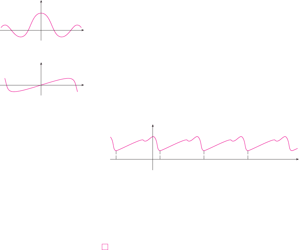
C. Symmetry

(i) If for all in , that is, the equation of the curve is unchanged

when is replaced by , then is an even function and the curve is symmetric about

the -axis. This means that our work is cut in half. If we know what the curve looks like

for , then we need only reﬂect about the -axis to obtain the complete curve [see

Figure 3(a)]. Here are some examples: , and .

(ii) If for all in , then is an odd function and the curve is

symmetric about the origin. Again we can obtain the complete curve if we know what

it looks like for . [Rotate 180° about the origin; see Figure 3(b).] Some simple

examples of odd functions are , and .

(iii) If for all in , where is a positive constant, then is called

a periodic function and the smallest such number is called the period. For instance,

has period and has period . If we know what the graph looks

like in an interval of length , then we can use translation to sketch the entire graph (see

Figure 4).

D. Asymptotes

(i) Horizontal Asymptotes. Recall from Section 4.4 that if either

then the line is a horizontal asymptote of the curve .

If it turns out that (or ), then we do not have an asymptote to the

right, but that is still useful information for sketching the curve.

(ii) Vertical Asymptotes. Recall from Section 2.2 that the line is a vertical

asymptote if at least one of the following statements is true:

(For rational functions you can locate the vertical asymptotes by equating the denomi-

nator to 0 after canceling any common factors. But for other functions this method does

not apply.) Furthermore, in sketching the curve it is very useful to know exactly which

of the statements in (1) is true. If is not deﬁned but is an endpoint of the domain

of , then you should compute or , whether or not this limit is

inﬁnite.

(iii) Slant Asymptotes. These are discussed at the end of this section.

E. Intervals of Increase or Decrease Use the I/D Test. Compute and ﬁnd the intervals

on which is positive ( is increasing) and the intervals on which is negative

( is decreasing).f

f !!x"ff !!x"

f !!x"

lim

x l a

" f !x"lim

x l a

f !x"f

af !a"

lim

f !x" ! #$ lim

f !x" ! #$

lim

f !x" ! $ lim

f !x" ! $

x ! a

#$lim

x l $

f !x" ! $

y ! f !x"y ! Llim

x l# $

f !x" ! L

lim

x l $

f !x" ! L

FIG URE 4

Periodic function:

translational symmetry

a-p a a+p a+2p

y ! tan x2

y ! sin x

fpDxf !x " p" ! f !x"

y ! sin xy ! x, y ! x

, y ! x

x & 0

fDxf !#x" ! #f !x"

y ! cos xy ! x

, y ! x

, y !

yx & 0

f#xx

Dxf !#x" ! f !x"

xy ! 0x

yf !0"y

244

|| ||

CHAPTER 4 APPLICATIONS OF DIFFERENTIATION

FIG URE 3

(a) Even function: reﬂectional symmetry

(b) Odd function: rotational symmetry

F. Local Maximum and Minimum Values Find the critical numbers of [the numbers

where or does not exist]. Then use the First Derivative Test. If

changes from positive to negative at a critical number , then is a local maximum.

If changes from negative to positive at , then is a local minimum. Although it

is usually preferable to use the First Derivative Test, you can use the Second Derivative

Test if and . Then implies that is a local minimum,

whereas implies that is a local maximum.

G. Concavity and Points of Inﬂection Compute and use the Concavity Test. The curve

is concave upward where and concave downward where . Inﬂec-

tion points occur where the direction of concavity changes.

H. Sketch the Curve Using the information in items A–G, draw the graph. Sketch the

asymptotes as dashed lines. Plot the intercepts, maximum and minimum points, and

inﬂection points. Then make the curve pass through these points, rising and falling

according to E, with concavity according to G, and approaching the asymptotes. If addi-

tional accuracy is desired near any point, you can compute the value of the derivative

there. The tangent indicates the direction in which the curve proceeds.

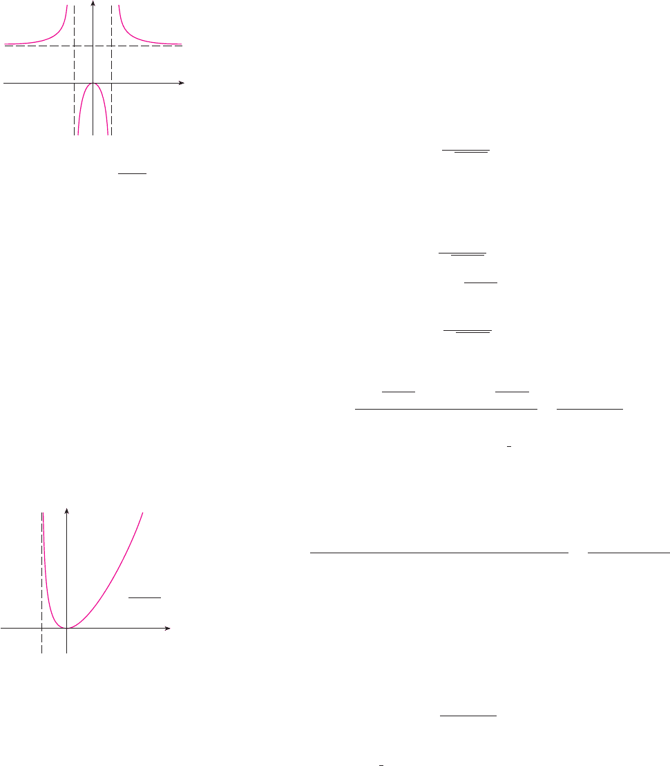
EXAMPLE 1 Use the guidelines to sketch the curve .

A. The domain is

B. The - and -intercepts are both 0.

C. Since , the function is even. The curve is symmetric about the -axis.

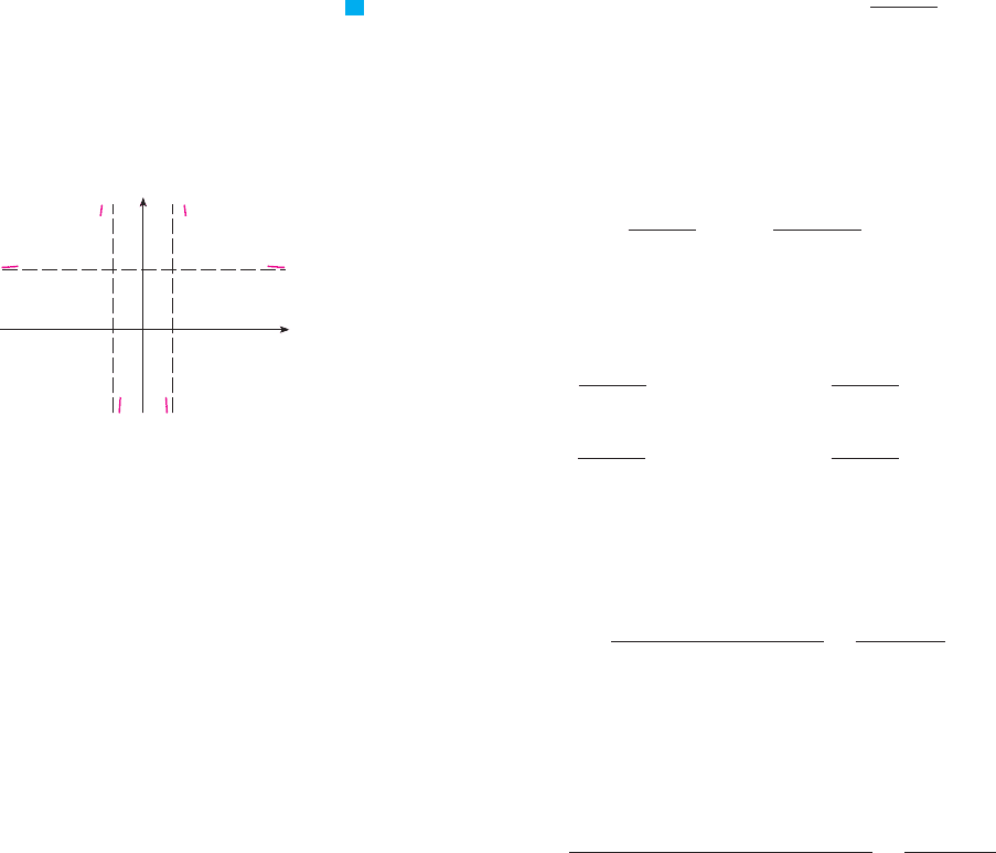
Therefore the line is a horizontal asymptote.

Since the denominator is 0 when , we compute the following limits:

Therefore the lines and are vertical asymptotes. This information

about limits and asymptotes enables us to draw the preliminary sketch in Figure 5,

showing the parts of the curve near the asymptotes.

Since when and when , is

increasing on and and decreasing on and .

F. The only critical number is . Since changes from positive to negative at 0,

is a local maximum by the First Derivative Test.

f '!x" !

#4!x

# 1"

" 4x ! 2!x

# 1"2x

# 1"

12x

" 4

# 1"

f !0" ! 0

f !x ! 0

!1, $"!0, 1"!#1, 0"!#$, #1"

f!x " 1"x ( 0f !!x"

)

0!x " #1"x

)

0f !!x" ( 0

f !!x" !

4x!x

# 1" # 2x

! 2x

# 1"

#4x

# 1"

x ! #1x ! 1

lim

# 1

! #$ lim

# 1

! $

lim

# 1

! $

lim

# 1

! #$

x ! *1

y ! 2

lim

x l*$

# 1

! lim

x l*$

1 # 1$x

! 2

yff !#x" ! f !x"

# 1 " 0& ! %x

x " *1& ! !#$, #1" " !#1, 1" " !1, $"

y !

# 1

f '!x"

)

0f '!x" ( 0

f '!x"

f !c"f '!c"

)

f !c"f '!c" ( 0f '!c" " 0f !!c" ! 0

f !c"cf !

f !c"c

f !f !!c"f !!c" ! 0

SECTION 4.5 SUMMARY OF CURVE SKETCHING

|| ||

245

FIG URE 5

Preliminary sketch

x=1x=_1

y=2

N We have shown the curve approaching its

horizontal asymptote from above in Figure 5.

This is conﬁrmed by the intervals of increase and

decrease.

Since for all , we have

and . Thus the curve is concave upward on the intervals

and and concave downward on . It has no point of inﬂection

since 1 and are not in the domain of .

H. Using the information in E–G, we ﬁnish the sketch in Figure 6. M

EXAMPLE 2 Sketch the graph of .

A. Domain

B. The - and -intercepts are both 0.

C. Symmetry: None

D. Since

there is no horizontal asymptote. Since as and is always

positive, we have

and so the line is a vertical asymptote.

We see that when

(

notice that is not in the domain of

)

, so the

only critical number is 0. Since when and when

, is decreasing on and increasing on .

F. Since and changes from negative to positive at 0, is a local

(and absolute) minimum by the First Derivative Test.

Note that the denominator is always positive. The numerator is the quadratic

, which is always positive because its discriminant is ,

which is negative, and the coefﬁcient of is positive. Thus for all in the

domain of , which means that is concave upward on and there is no point

of inﬂection.

H. The curve is sketched in Figure 7.

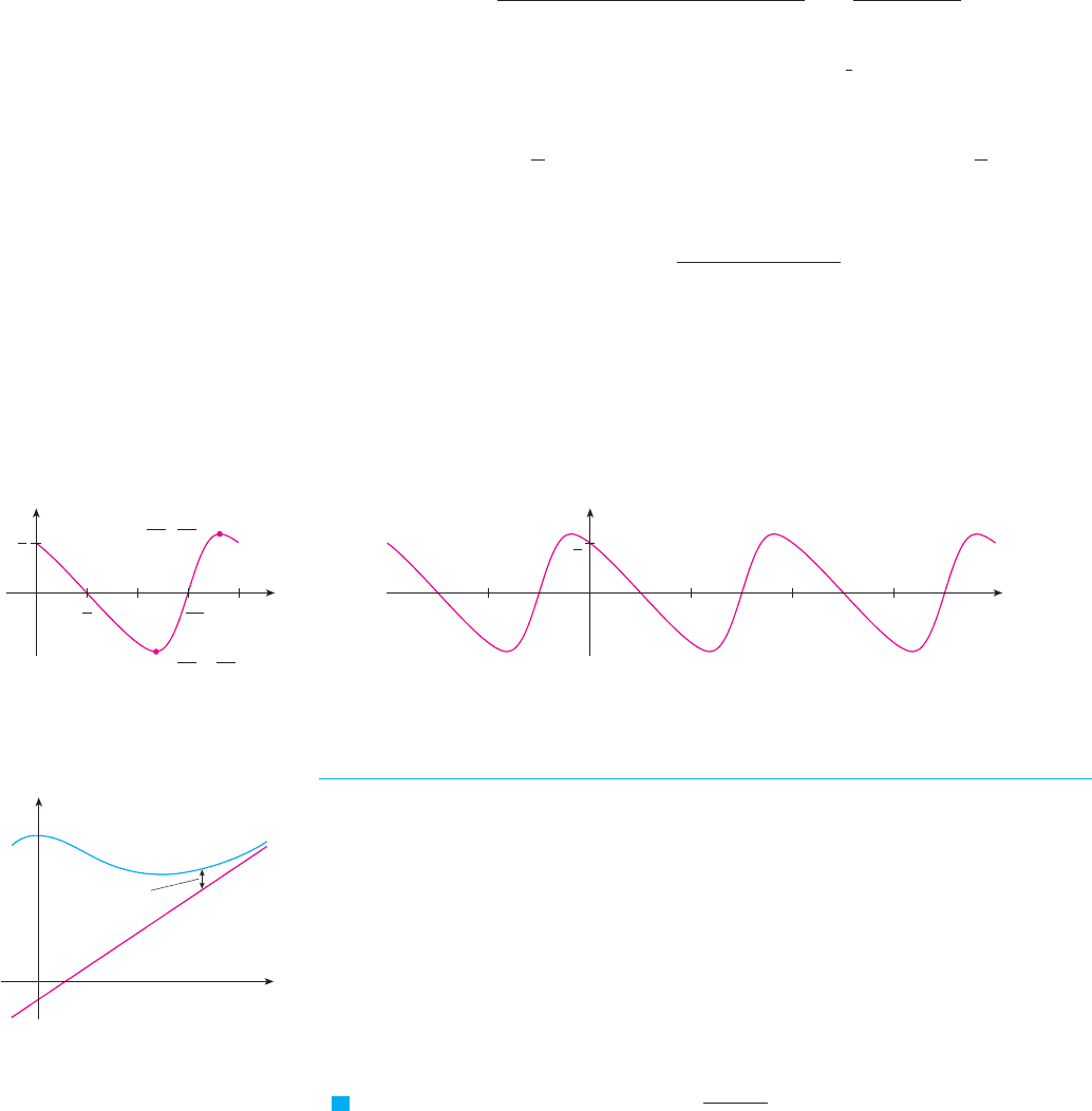
EXAMPLE 3 Sketch the graph of .

A. The domain is .

B. The -intercept is . The -intercepts occur when , that is,

, where is an integer.

C. is neither even nor odd, but for all and so is periodic and

has period . Thus, in what follows, we need to consider only and then

extend the curve by translation in part H.

0 + x + 2

fxf !x " 2

" ! f !x"f

nx ! !2n " 1"

cos x ! 0xf !0" !

f !x" !

cos x

2 " sin x

!#1, $"ff

xf '!x" ( 0x

# 4ac ! #323x

" 8x " 8

f '!x" !

2!x " 1"

3$2

!6x " 4" # !3x

" 4x"3!x " 1"

1$2

4!x " 1"

" 8x " 8

4!x " 1"

5$2

f !0" ! 0f !f !!0" ! 0

!0, $"!#1, 0"fx ( 0

f !!x" ( 0#1

)

0f !!x"

)

x ! 0f !!x" ! 0

f !!x" !

x " 1 # x

! 1$

(

x " 1

)

x " 1

x!3x " 4"

2!x " 1"

3$2

x ! #1

lim

x " 1

! $

f !x"x l #1

x " 1 l 0

lim

x l $

x " 1

! $

! %x

x " 1 ( 0& ! %x

x ( #1& ! !#1, $"

f !x" !

x " 1

f#1

!#1, 1"!1, $"!#$, #1"

f '!x"

)

0 &?

)

( 1&?x

# 1 ( 0&?f '!x" ( 0

x12x

" 4 ( 0

246

|| ||

CHAPTER 4 APPLICATIONS OF DIFFERENTIATION

FIG URE 6

Finished sketch of y=

x=1x=_1

y=2

2≈

≈-1

FIG URE 7

x=_1

œ„„„„

≈

x+1

D. Asymptotes: None

Thus when

. So is increasing on and decreasing on

and .

F. From part E and the First Derivative Test, we see that the local minimum value

is and the local maximum value is .

G. If we use the Quotient Rule again and simplify, we get

Because and for all , we know that when

, that is, . So is concave upward on and

concave downward on and . The inﬂection points are

H. The graph of the function restricted to is shown in Figure 8. Then we

extend it, using periodicity, to the complete graph in Figure 9.

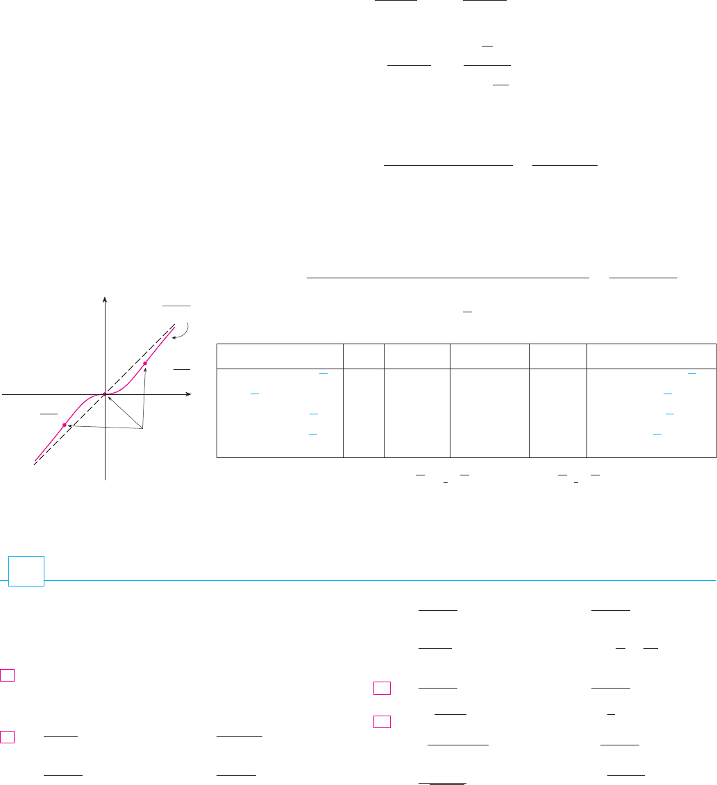
SLANT AS Y M P TOTES

Some curves have asymptotes that are oblique, that is, neither horizontal nor vertical. If

then the line is called a slant asymptote because the vertical distance

between the curve and the line approaches 0, as in Figure 10. (A

similar situation exists if we let .) For rational functions, slant asymptotes occur

when the degree of the numerator is one more than the degree of the denominator. In such

a case the equation of the slant asymptote can be found by long division as in the follow-

ing example.

EXAMPLE 4 Sketch the graph of .

A. The domain is .

B. The - and -intercepts are both 0.

C. Since , is odd and its graph is symmetric about the origin.ff !#x" ! #f !x"

! ! !#$, $"

f !x" !

" 1

x l #$

y ! mx " by ! f !x"

y ! mx " b

lim

x l $

' f !x" # !mx " b"( ! 0

FIG URE 8

2π

3π

” , ’

11π

œ„3

”

7π

œ„3

’

FIG URE 9

π_π

2π 3π

0 + x + 2

and !3

$2, 0"

$2, 0"!3

$2, 2

"!0,

$2"

$2, 3

$2"f

)

$2cos x

)

f '!x" ( 0x1 # sin x & 0!2 " sin x"

( 0

f '!x" ! #

2 cos x !1 # sin x"

!2 " sin x"

f !11

$6" ! 1$

f !7

$6" ! #1$

!11

$6, 2

!0, 7

$6"!7

$6, 11

$6"f7

)

2 sin x " 1

)

0 &? sin x

)

&?f !!x" ( 0

f !!x" !

!2 " sin x"!#sin x" # cos x !cos x"

!2 " sin x"

! #

2 sin x " 1

!2 " sin x"

SECTION 4.5 SUMMARY OF CURVE SKETCHING

|| ||

247

FIG URE 10

y=ƒ

y=mx+b

ƒ-(mx+b)

D. Since is never 0, there is no vertical asymptote. Since as and

as , there is no horizontal asymptote. But long division gives

So the line is a slant asymptote.

Since for all (except 0), is increasing on .

F. Although , does not change sign at 0, so there is no local maximum or

minimum.

Since when or , we set up the following chart:

The points of inﬂection are , and .

H. The graph of is sketched in Figure 11. M

(

)(

, #

)

, !0, 0"

x ! *

x ! 0f '!x" ! 0

f '!x" !

!4x

" 6x"!x

" 1"

# !x

" 3x

" ! 2!x

" 1"2x

" 1"

2x!3 # x

" 1"

f !f !!0" ! 0

!#$, $"fxf !!x" ( 0

f !!x" !

" 1" # x

! 2x

" 1"

" 3"

" 1"

y ! x

x l *$ f !x" # x ! #

" 1

! #

1 "

l 0

f !x" !

" 1

! x #

" 1

x l #$f !x" l #$

x l $f !x" l $x

" 1

248

|| ||

CHAPTER 4 APPLICATIONS OF DIFFERENTIATION

Interval x f

# # " " CU on

# " " # CD on

" " " " CU on

" # " # CD on

(

, $

)

x (

(

)

(

, 0

)

(

#$, #

)

f '!x"!x

" 1"

3 # x

FIG URE 11

y=x

”

_œ„3,_ ’

3œ

„

inflection

points

≈+1

”œ„3, ’

3œ

„

13. 14.

15. 16.

18.

20.

21. 22.

23. 24.

y ! x

2 # x

y !

" 1

y !

" x

# xy !

" x # 2

y ! 2

# xy ! x

5 # x

19.

y !

# 1

y !

" 3

17.

y ! 1 "

y !

x # 1

y !

" 9

y !

" 9

1–38 Use the guidelines of this section to sketch the curve.

1. 2.

3. 4.

7. 8.

10.

11. 12.

y !

# 9

y !

# 9

y !

# 4

# 2x

y !

x # 1

y ! !4 # x

y ! 2x

# 5x

" 1

y ! x!x " 2"

y ! x

" 4x

y ! 8x

# x

y ! 2 # 15x " 9x

# x

y ! x

" 6x

" 9xy ! x

" x

E X E R C I S E S

4.5

SECTION 4.5 SUMMARY OF CURVE SKETCHING

|| ||

249

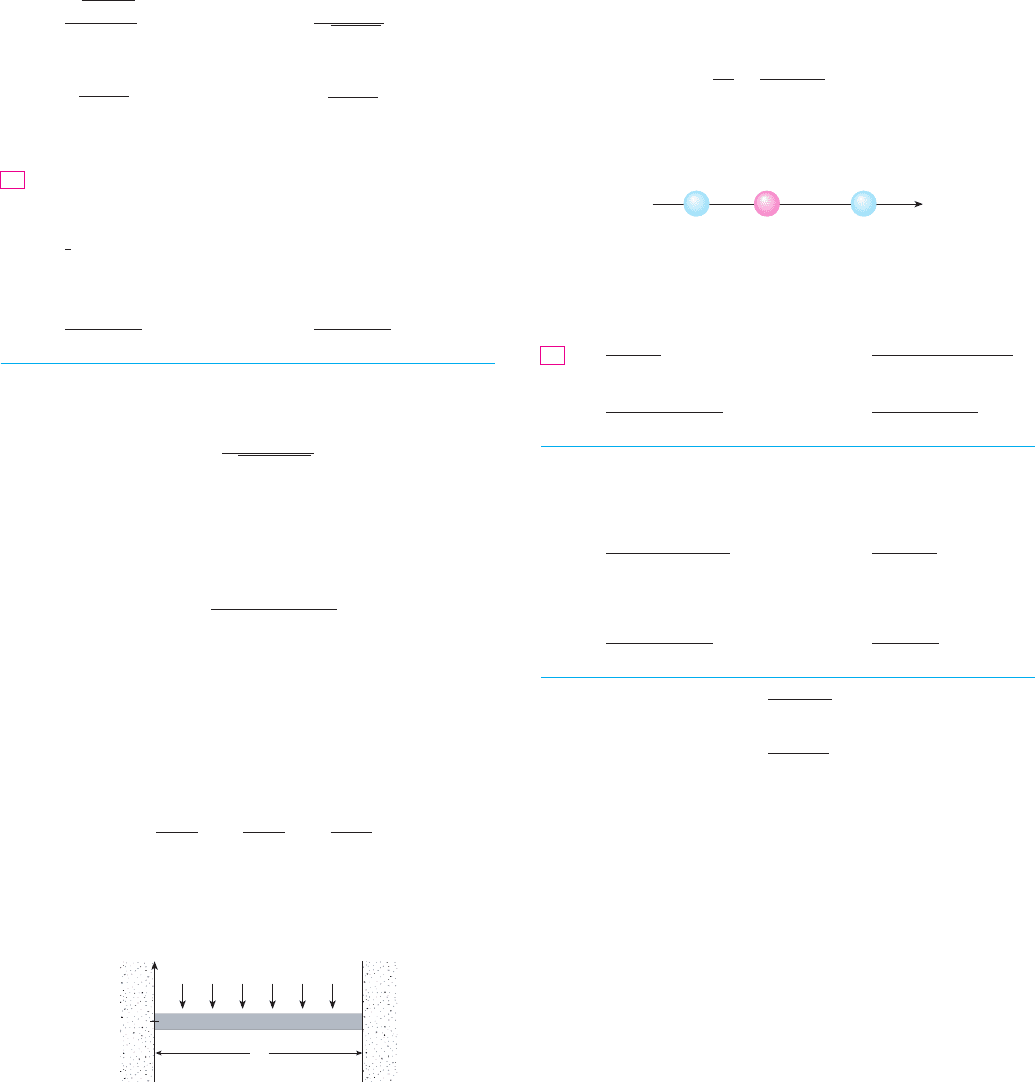
charge at a position between them. It follows from Cou-

lomb’s Law that the net force acting on the middle particle is

where is a positive constant. Sketch the graph of the net force

function. What does the graph say about the force?

43– 46 Find an equation of the slant asymptote. Do not sketch the

curve.

44.

45. 46.

47–52 Use the guidelines of this section to sketch the curve. In

guideline D ﬁnd an equation of the slant asymptote.

47. 48.

49. 50.

51. 52.

53. Show that the curve has two slant asymptotes:

and . Use this fact to help sketch the curve.

54. Show that the curve has two slant asymptotes:

and . Use this fact to help sketch the

curve.

55. Show that the lines and are slant

asymptotes of the hyperbola .

56. Let . Show that

This shows that the graph of approaches the graph of

, and we say that the curve is asymptotic to

the parabola . Use this fact to help sketch the

graph of .

57. Discuss the asymptotic behavior of in the

same manner as in Exercise 56. Then use your results to help

sketch the graph of .

58. Use the asymptotic behavior of to sketch

its graph without going through the curve-sketching procedure

of this section.

f !x" ! cos x " 1$x

f !x" ! !x

" 1"$x

y ! x

y ! f !x"y ! x

lim

x l*$

' f !x" # x

( ! 0

f !x" ! !x

" 1"$x

" # !y

" ! 1

y ! #!b$a"xy ! !b$a"x

y ! #x # 2y ! x " 2

y !

" 4x

y ! #2xy ! 2x

y !

" 9

y !

!x " 1"

!x # 1"

y !

" x

" 1

xy ! x

" x " 1xy ! x

" 4

y !

" 12

x # 2

y !

#2x

" 5x # 1

2x # 1

y !

" x

# x

" 2

y !

# 2x

" 5

" x # 3

y !

" x

" x " 3

" 2x

y !

" 1

x " 1

43.

F!x" ! #

!x # 2"

)

x#1

25. 26.

27. 28.

29. 30.

31. 32.

34. ,

35. ,

36. ,

37. 38.

39. In the theory of relativity, the mass of a particle is

where is the rest mass of the particle, is the mass when

the particle moves with speed relative to the observer, and

is the speed of light. Sketch the graph of as a function of .

40. In the theory of relativity, the energy of a particle is

where is the rest mass of the particle, is its wave length,

and is Planck’s constant. Sketch the graph of as a function

of . What does the graph say about the energy?

41. The ﬁgure shows a beam of length embedded in concrete

walls. If a constant load is distributed evenly along its

length, the beam takes the shape of the deﬂection curve

where and are positive constants. ( is Young’s modulus of

elasticity and is the moment of inertia of a cross-section of

the beam.) Sketch the graph of the deﬂection curve.

42. Coulomb’s Law states that the force of attraction between two

charged particles is directly proportional to the product of the

charges and inversely proportional to the square of the distance

between them. The ﬁgure shows particles with charge 1 located

at positions 0 and 2 on a coordinate line and a particle with

EIE

y ! #

24EI

12EI

24EI

E !

" h

m !

1 # v

y !

sin x

2 " cos x

y !

sin x

1 " cos x

)

$2y ! sec x " tan x

)

y !

x # sin x

)

y ! 2x # tan x

)

y ! x tan x

33.

y ! x " cos xy ! 3 sin x # sin

y !

" 1y !

# 1

y ! x

5$3

# 5x

2$3

y ! x # 3x

1$3

y !

# 1

y !

1 # x

GRA PHIN G WI TH C A L CUL US A ND C ALCU LATOR S

The method we used to sketch curves in the preceding section was a culmination of much

of our study of differential calculus. The graph was the ﬁnal object that we produced. In

this section our point of view is completely different. Here we start with a graph produced

by a graphing calculator or computer and then we reﬁne it. We use calculus to make sure

that we reveal all the important aspects of the curve. And with the use of graphing devices

we can tackle curves that would be far too complicated to consider without technology.

The theme is the interaction between calculus and calculators.

EXAMPLE 1 Graph the polynomial . Use the graphs of

and to estimate all maximum and minimum points and intervals of concavity.

SOLUTION If we specify a domain but not a range, many graphing devices will deduce a

suitable range from the values computed. Figure 1 shows the plot from one such device

if we specify that . Although this viewing rectangle is useful for showing

that the asymptotic behavior (or end behavior) is the same as for , it is obviously

hiding some ﬁner detail. So we change to the viewing rectangle by

shown in Figure 2.

From this graph it appears that there is an absolute minimum value of about 3

when (by using the cursor) and is decreasing on and increas-

ing on . Also, there appears to be a horizontal tangent at the origin and inﬂec-

tion points when and when is somewhere between and .

Now let’s try to conﬁrm these impressions using calculus. We differentiate and get

When we graph in Figure 3 we see that changes from negative to positive when

; this conﬁrms (by the First Derivative Test) the minimum value that we

found earlier. But, perhaps to our surprise, we also notice that changes from posi-

tive to negative when and from negative to positive when . This means

that has a local maximum at 0 and a local minimum when , but these were

hidden in Figure 2. Indeed, if we now zoom in toward the origin in Figure 4, we see

what we missed before: a local maximum value of 0 when and a local minimum

value of about when .

What about concavity and inﬂection points? From Figures 2 and 4 there appear to be

inﬂection points when is a little to the left of and when is a little to the right of 0.

But it’s difﬁcult to determine inﬂection points from the graph of , so we graph the sec-f

x#1x

_3 2

y=fª(x)

FIG URE 3

_1 1

y=ƒ

FIG URE 4

x ) 0.35#0.1

x ! 0

x ) 0.35f

x ) 0.35x ! 0

f !!x"

x ) #1.62

f !!x"f !

f '!x" ! 60x

" 60x

" 18x # 4

f !!x" ! 12x

" 15x

" 9x

# 4x

#1#2xx ! 0

!#1.62, $"

!#$, #1.62"fx ) #1.62

#15.3

'#50, 100('#3, 2(

y ! 2x

#5 + x + 5

f '

f !f !x" ! 2x

" 3x

# 2x

4. 6

250

|| ||

CHAPTER 4 APPLICATIONS OF DIFFERENTIATION

41,000

_1000

_5 5

y=ƒ

FIG URE 1

100

_50

_3 2

y=ƒ

FIG URE 2

N If you have not already read Section 1.4, you

should do so now. In particular, it explains how

to avoid some of the pitfalls of graphing devices

by choosing appropriate viewing rectangles.

ond derivative in Figure 5. We see that changes from positive to negative when

and from negative to positive when . So, correct to two decimal

places, is concave upward on and and concave downward on

. The inﬂection points are and .

We have discovered that no single graph reveals all the important features of this

polynomial. But Figures 2 and 4, when taken together, do provide an accurate picture. M

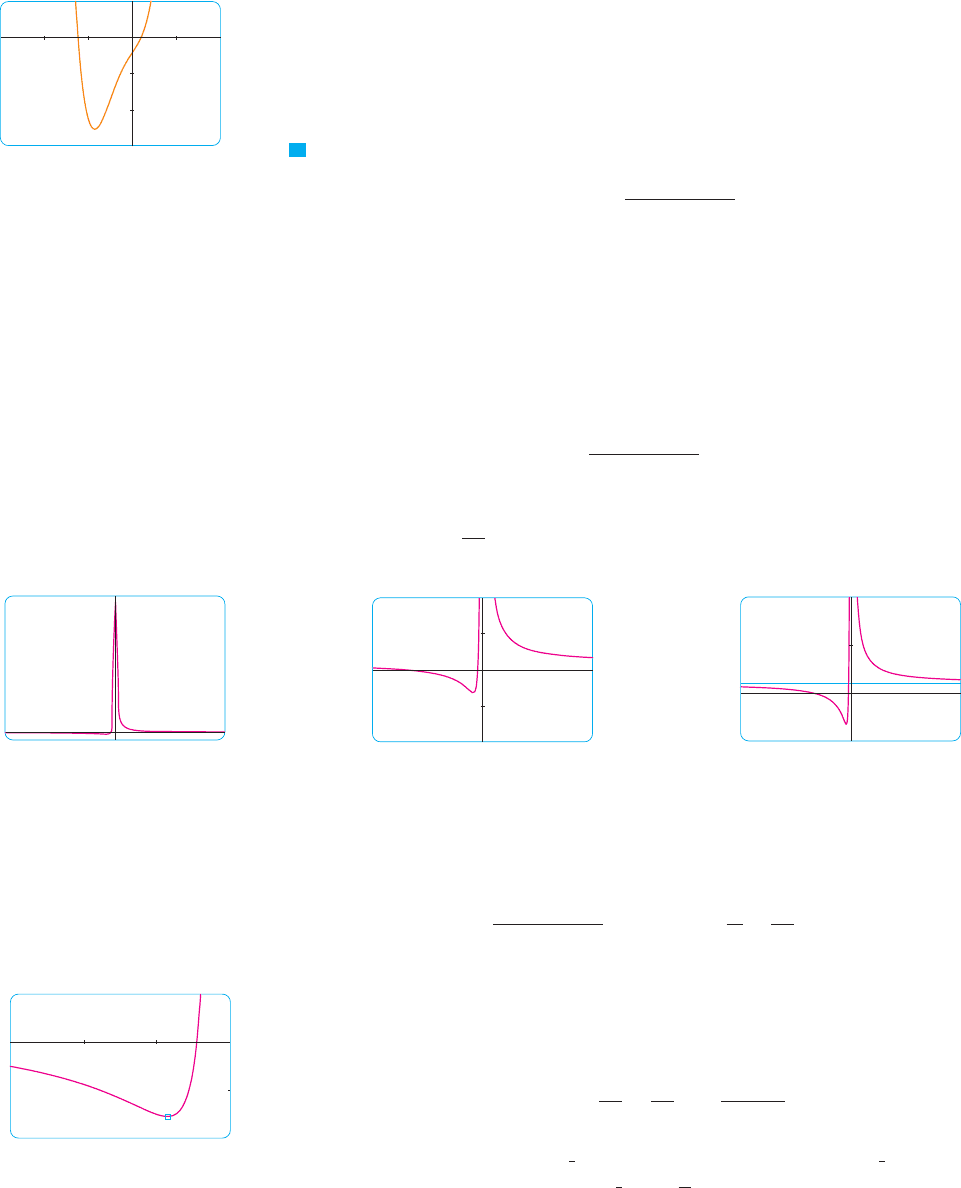
EXAMPLE 2 Draw the graph of the function

in a viewing rectangle that contains all the important features of the function. Estimate

the maximum and minimum values and the intervals of concavity. Then use calculus to

ﬁnd these quantities exactly.

SOLUTION Figure 6, produced by a computer with automatic scaling, is a disaster. Some

graphing calculators use by as the default viewing rectangle, so let’s

try it. We get the graph shown in Figure 7; it’s a major improvement.

The -axis appears to be a vertical asymptote and indeed it is because

Figure 7 also allows us to estimate the -intercepts: about and . The exact val-

ues are obtained by using the quadratic formula to solve the equation ;

we get .

To get a better look at horizontal asymptotes, we change to the viewing rectangle

by in Figure 8. It appears that is the horizontal asymptote and

this is easily conﬁrmed:

To estimate the minimum value we zoom in to the viewing rectangle by

in Figure 9. The cursor indicates that the absolute minimum value is about

when , and we see that the function decreases on and and

increases on . The exact values are obtained by differentiating:

This shows that when and when and when

. The exact minimum value is .f

(

)

! #

) #3.08x ( 0

)

f !!x"

)

0f !!x" ( 0

f !!x" ! #

! #

7x " 6

!#0.9, 0"

!0, $"!#$, #0.9"x ) #0.9

#3.1'#4, 2(

'#3, 0(

lim

x l*$

" 7x " 3

! lim

x l*$

1 "

! 1

y ! 1'#5, 10('#20, 20(

3 - 10!*

_5 5

y=ƒ

FIG URE 6

_10

_10 10

y=ƒ

FIG URE 7

_20 20

y=ƒ

y=1

FIG URE 8

x !

(

#7 *

)

" 7x " 3 ! 0

#6.5#0.5x

lim

x l 0

" 7x " 3

! $

'#10, 10('#10, 10(

f !x" !

" 7x " 3

!0.19, #0.05"!#1.23, #10.18"!#1.23, 0.19"

!0.19, $"!#$, #1.23"f

x ) 0.19x ) #1.23

f 'f '

SECTION 4.6 GRAPHING WITH CALCULUS AND CALCULATORS

|| ||

251

_30

_3 2

y=f·(x)

FIG URE 5

_3 0

y=ƒ

FIG URE 9