Stewart J. Calculus

Подождите немного. Документ загружается.

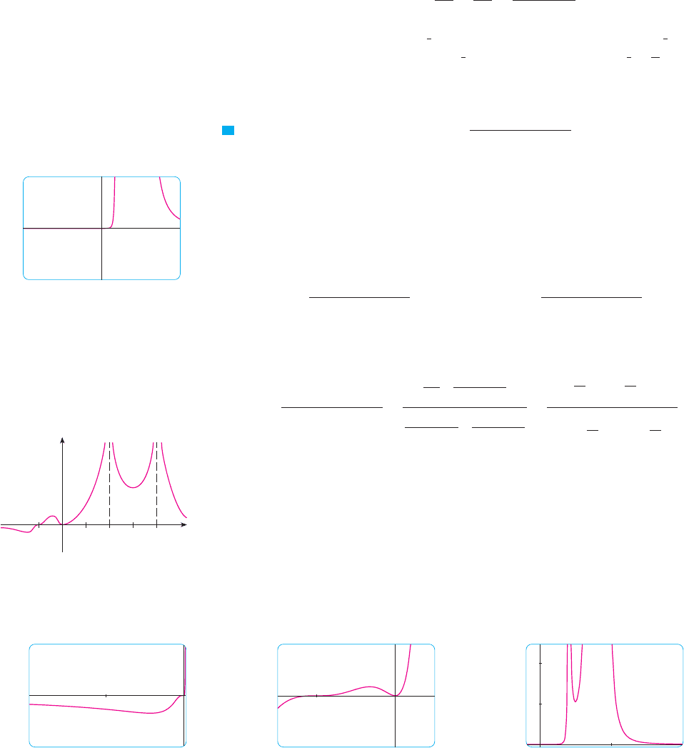
Figure 9 also shows that an inﬂection point occurs somewhere between and

. We could estimate it much more accurately using the graph of the second deriv-

ative, but in this case it’s just as easy to ﬁnd exact values. Since

we see that when . So is concave upward on and

and concave downward on . The inﬂection point is .

The analysis using the ﬁrst two derivatives shows that Figures 7 and 8 display all the

major aspects of the curve.

EXAMPLE 3 Graph the function .

SOLUTION Drawing on our experience with a rational function in Example 2, let’s start by

graphing in the viewing rectangle by . From Figure 10 we have

the feeling that we are going to have to zoom in to see some ﬁner detail and also zoom

out to see the larger picture. But, as a guide to intelligent zooming, let’s ﬁrst take a close

look at the expression for . Because of the factors and in the

denominator, we expect and to be the vertical asymptotes. Indeed

To ﬁnd the horizontal asymptotes, we divide numerator and denominator by :

This shows that , so the -axis is a horizontal asymptote.

It is also very useful to consider the behavior of the graph near the -intercepts using

an analysis like that in Example 11 in Section 4.4. Since is positive, does not

change sign at 0 and so its graph doesn’t cross the -axis at 0. But, because of the factor

, the graph does cross the -axis at and has a horizontal tangent there.

Putting all this information together, but without using derivatives, we see that the curve

has to look something like the one in Figure 11.

Now that we know what to look for, we zoom in (several times) to produce the graphs

in Figures 12 and 13 and zoom out (several times) to get Figure 14.

0.05

_0.05

_100 1

y=ƒ

FIG URE 12

0.0001

_0.0001

_1.5 0.5

y=ƒ

FIG URE 13

500

_10

_1 10

y=ƒ

FIG URE 14

#1x!x " 1"

f !x"x

xf !x" l 0 as x l *$

!x " 1"

!x # 2"

!x # 4"

!x " 1"

!x # 2"

!x # 4"

1 "

1 #

lim

x l 4

!x " 1"

!x # 2"

!x # 4"

! $andlim

x l 2

!x " 1"

!x # 2"

!x # 4"

! $

x ! 4x ! 2

!x # 4"

!x # 2"

f !x"

'#10, 10('#10, 10(f

f !x" !

!x " 1"

!x # 2"

!x # 4"

(

, #

)(

#$, #

)

!0, $"

(

, 0

)

f!x " 0"x ( #

f '!x" ( 0

f '!x" !

2(7x " 9"

x ! #2

x ! #1

252

|| ||

CHAPTER 4 APPLICATIONS OF DIFFERENTIATION

_10

_10 10

y=ƒ

FIG URE 10

FIG URE 11

1 2 3_1 4

We can read from these graphs that the absolute minimum is about and occurs

when . There is also a local maximum when and a local

minimum when . These graphs also show three inﬂection points near

and and two between and . To estimate the inﬂection points closely we

would need to graph , but to compute by hand is an unreasonable chore. If you

have a computer algebra system, then it’s easy to do (see Exercise 13).

We have seen that, for this particular function, three graphs (Figures 12, 13, and 14)

are necessary to convey all the useful information. The only way to display all these

features of the function on a single graph is to draw it by hand. Despite the exaggera-

tions and distortions, Figure 11 does manage to summarize the essential nature of the

function.

EXAMPLE 4 Graph the function . For , estimate all

maximum and minimum values, intervals of increase and decrease, and inﬂection points

correct to one decimal place.

SOLUTION We ﬁrst note that is periodic with period . Also, is odd and

for all . So the choice of a viewing rectangle is not a problem for this function: We start

with by . (See Figure 15.)

It appears that there are three local maximum values and two local minimum values in

that window. To conﬁrm this and locate them more accurately, we calculate that

and graph both and in Figure 16.

Using zoom-in and the First Derivative Test, we ﬁnd the following values to one deci-

mal place.

The second derivative is

f '!x" ! #!1 " 2 cos 2x"

sin!x " sin 2x" # 4 sin 2x cos!x " sin 2x"

Local minimum values: f !1.0" ) 0.94, f !2.1" ) 0.94

Local maximum values: f !0.6" ) 1, f !1.6" ) 1, f !2.5" ) 1

Intervals of decrease: !0.6, 1.0", !1.6, 2.1", !2.5,

Intervals of increase: !0, 0.6", !1.0, 1.6", !2.1, 2.5"

f !f

f !!x" ! cos!x " sin 2x" ! !1 " 2 cos 2x"

1.1

_1.1

FIG URE 15

1.2

_1.2

y=ƒ

y=fª(x)

FIG URE 16

'#1.1, 1.1('0,

(

f !x"

+ 1f2

0 + x +

f !x" ! sin!x " sin 2x"

f 'f '

0#1#1#5,

#35,x ) 2.5)211

x ) #0.3)0.00002x ) #20

#0.02

SECTION 4.6 GRAPHING WITH CALCULUS AND CALCULATORS

|| ||

253

N The family of functions

where is a constant, occurs in applications to

frequency modulation (FM) synthesis. A sine

wave is modulated by a wave with a different

frequency . The case where is

studied in Example 4. Exercise 19 explores

another special case.

c ! 2!sin cx"

f !x" ! sin!x " sin cx"

Graphing both and in Figure 17, we obtain the following approximate values:

Having checked that Figure 15 does indeed represent accurately for ,

we can state that the extended graph in Figure 18 represents accurately for

. M

Our ﬁnal example is concerned with families of functions. As discussed in Section 1.4,

this means that the functions in the family are related to each other by a formula that con-

tains one or more arbitrary constants. Each value of the constant gives rise to a member of

the family and the idea is to see how the graph of the function changes as the constant

changes.

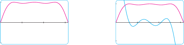
EXAMPLE 5 How does the graph of vary as varies?

SOLUTION The graphs in Figures 19 and 20 (the special cases and ) show

two very different-looking curves. Before drawing any more graphs, let’s see what mem-

bers of this family have in common. Since

for any value of , they all have the -axis as a horizontal asymptote. A vertical asymp-

tote will occur when . Solving this quadratic equation, we get

. When , there is no vertical asymptote (as in Figure 19). When

, the graph has a single vertical asymptote because

When

there are two vertical asymptotes: (as in Figure 20).

Now we compute the derivative:

This shows that when (if ), when , and

when . For , this means that increases on

and decreases on . For , there is an absolute maximum value

. For , is a local maximum value and the

intervals of increase and decrease are interrupted at the vertical asymptotes.

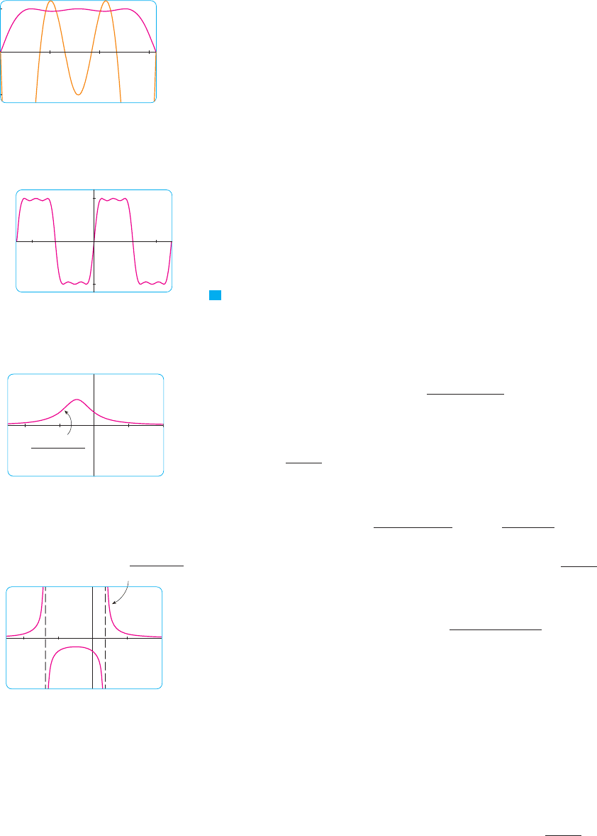
Figure 21 is a “slide show” displaying ﬁve members of the family, all graphed in the

viewing rectangle by . As predicted, is the value at which a transi-

tion takes place from two vertical asymptotes to one, and then to none. As increases

from , we see that the maximum point becomes lower; this is explained by the fact that

as . As decreases from , the vertical asymptotes become more

widely separated because the distance between them is , which becomes large2

1 ! c

1cc l "1!"c ! 1# l 0

c ! 1$!2, 2%$!5, 4%

f "!1# ! 1!"c ! 1#c

1f "!1# ! 1!"c ! 1#

c $ 1"!1, "#

"!", !1#fc % 1x $ !1f &"x#

!1f &"x# $ 0c " 1x ! !1f &"x# ! 0

f &"x# ! !

2x ' 2

' 2x ' c#

x ! !1 (

1 ! c

lim

x l !1

' 2x ' 1

! lim

x l !1

"x ' 1#

! "

x ! !1c ! 1

c $ 1x ! !1 (

1 ! c

' 2x ' c ! 0

lim

x l("

' 2x ' c

! 0

c ! !2c ! 2

cf "x# ! 1!"x

' 2x ' c#

)

* x * 2

)

0 * x *

)

Inflection points: "0, 0#, "0.8, 0.97#, "1.3, 0.97#, "1.8, 0.97#, "2.3, 0.97#

Concave downward on: "0, 0.8#, "1.3, 1.8#, "2.3,

)

Concave upward on: "0.8, 1.3#, "1.8, 2.3#

f +f

254

|| ||

CHAPTER 4 APPLICATIONS OF DIFFERENTIATION

FIG URE 19

c=2

≈+2x+2

_5 4

1.2

_1.2

0 π

f ·

FIG URE 17

1.2

_1.2

_2π 2π

FIG URE 18

FIG URE 20

c=_2

_5 4

≈+2x-2

as . Again, the maximum point approaches the -axis because

as .

There is clearly no inﬂection point when . For we calculate that

and deduce that inﬂection points occur when . So the inﬂection

points become more spread out as increases and this seems plausible from the last two

parts of Figure 21.

x ! !1 (

3"c ! 1#!3

f +"x# !

2"3x

' 6x ' 4 ! c#

' 2x ' c#

c $ 1c * 1

c=3c=2c=1c=0c=_1

FIG URE 21 The family of functions ƒ=1/(≈+2x+c)

c l !"

1!"c ! 1# l 0xc l !"

SECTION 4.6 GRAPHING WITH CALCULUS AND CALCULATORS

|| ||

255

See an animation of Figure 21 in

Visual 4.4.

TE C

11–12 Sketch the graph by hand using asymptotes and intercepts,

but not derivatives. Then use your sketch as a guide to producing

graphs (with a graphing device) that display the major features of

the curve. Use these graphs to estimate the maximum and mini-

mum values.

12.

13. If is the function considered in Example 3, use a computer

algebra system to calculate and then graph it to conﬁrm

that all the maximum and minimum values are as given in the

example. Calculate and use it to estimate the intervals of

concavity and inﬂection points.

14. If is the function of Exercise 12, ﬁnd and and use their

graphs to estimate the intervals of increase and decrease and

concavity of .

15–18 Use a computer algebra system to graph and to ﬁnd

and . Use graphs of these derivatives to estimate the intervals

of increase and decrease, extreme values, intervals of concavity,

and inﬂection points of .

15. 16.

17.

, x * 20f "x# !

x ' 5 sin x

f "x# !

2!3

1 ' x ' x

f "x# !

' x ' 1

f +

f &f

CAS

f +f &f

CAS

f +

f &

CAS

f "x# !

"2 x ' 3#

"x ! 2#

"x ! 5#

f "x# !

"x ' 4#"x ! 3#

"x ! 1#

11.

1–8 Produce graphs of that reveal all the important aspects of

the curve. In particular, you should use graphs of and to esti-

mate the intervals of increase and decrease, extreme values, inter-

vals of concavity, and inﬂection points.

8. ,

9–10 Produce graphs of that reveal all the important aspects of

the curve. Estimate the intervals of increase and decrease and inter-

vals of concavity, and use calculus to ﬁnd these intervals exactly.

10.

f "x# !

2 , 10

f "x# ! 1 '

)

* x * 2

)

f "x# !

sin x

!4 * x * 4f "x# ! x

! 4x ' 7 cos x

f "x# ! tan x ' 5 cos x

f "x# !

! x

! 4x ' 1

f "x# !

! 1

40x

' x ' 1

f "x# ! x

! 10x

! 400x

' 2500x

f "x# ! x

! 15x

' 75x

! 125x

! x

f "x# ! 4x

! 32x

' 89x

! 95x ' 29

f +f &

;

E X E R C I S E S

4.6

24. 25.

26.

Investigate the family of curves given by the equation

. Start by determining the transitional

value of at which the number of inﬂection points changes.

Then graph several members of the family to see what shapes

are possible. There is another transitional value of at which

the number of critical numbers changes. Try to discover it

graphically. Then prove what you have discovered.

27.

(a) Investigate the family of polynomials given by the equa-

tion . For what values of does

the curve have minimum points?

(b) Show that the minimum and maximum points of every

curve in the family lie on the parabola . Illus-

trate by graphing this parabola and several members of

the family.

28.

(a) Investigate the family of polynomials given by the equa-

tion . For what values of does

the curve have maximum and minimum points?

(b) Show that the minimum and maximum points of every

curve in the family lie on the curve . Illustrate

by graphing this curve and several members of the family.

y ! x ! x

cf "x# ! 2x

' cx

' 2 x

y ! 1 ! x

cf "x# ! cx

! 2 x

' 1

f "x# ! x

' cx

' x

f "x# ! cx ' sin xf "x# !

"1 ! x

' cx

18.

19.

In Example 4 we considered a member of the family of func-

tions that occur in FM synthesis. Here

we investigate the function with . Start by graphing in

the viewing rectangle by . How many local

maximum points do you see? The graph has more than are

visible to the naked eye. To discover the hidden maximum

and minimum points you will need to examine the graph of

very carefully. In fact, it helps to look at the graph of at

the same time. Find all the maximum and minimum values

and inﬂection points. Then graph in the viewing rectangle

by and comment on symmetry.

20–25

Describe how the graph of varies as varies. Graph

several members of the family to illustrate the trends that you dis-

cover. In particular, you should investigate how maximum and

minimum points and inﬂection points move when changes. You

should also identify any transitional values of at which the basic

shape of the curve changes.

20. 21.

22.

f "x# !

1 ' c

23.

f "x# ! x

! x

f "x# ! x

' cx

f "x# ! x

' cx

$!1.2, 1.2%$!2

)

, 2

)

f +f &

$!1.2, 1.2%$0,

)

fc ! 3

f "x# ! sin"x ' sin cx#

f "x# !

2x ! 1

' x ' 1

256

|| ||

CHAPTER 4 APPLICATIONS OF DIFFERENTIATION

OPTIMIZATION PROBLEMS

The methods we have learned in this chapter for ﬁnding extreme values have practical

applications in many areas of life. A businessperson wants to minimize costs and maxi-

mize proﬁts. A traveler wants to minimize transportation time. Fermat’s Principle in optics

states that light follows the path that takes the least time. In this section and the next we

solve such problems as maximizing areas, volumes, and proﬁts and minimizing distances,

times, and costs.

In solving such practical problems the greatest challenge is often to convert the word

problem into a mathematical optimization problem by setting up the function that is to be

maximized or minimized. Let’s recall the problem-solving principles discussed on page 54

and adapt them to this situation:

STEPS IN SOLVING OPTIMIZATION PROBLEMS

1. Understand the Problem

The ﬁrst step is to read the problem carefully until it is

clearly understood. Ask yourself: What is the unknown? What are the given quanti-

ties? What are the given conditions?

2. Draw a Diagram

In most problems it is useful to draw a diagram and identify the

given and required quantities on the diagram.

3. Introduce Notation Assign a symbol to the quantity that is to be maximized or

minimized (let’s call it for now). Also select symbols for other

unknown quantities and label the diagram with these symbols. It may help to use

initials as suggestive symbols—for example, for area, for height, for time.thA

"a, b, c, . . . , x, y#Q

4.7

Openmirrors.com

4. Express in terms of some of the other symbols from Step 3.

5. If has been expressed as a function of more than one variable in Step 4, use the

given information to ﬁnd relationships (in the form of equations) among these

variables. Then use these equations to eliminate all but one of the variables in the

expression for . Thus will be expressed as a function of one variable , say,

. Write the domain of this function.

6. Use the methods of Sections 4.1 and 4.3 to ﬁnd the absolute maximum or mini-

mum value of . In particular, if the domain of is a closed interval, then the

Closed Interval Method in Section 4.1 can be used.

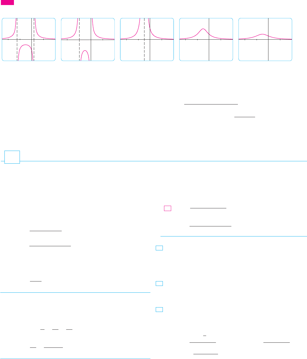
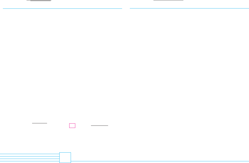
EXAMPLE 1 A farmer has 2400 ft of fencing and wants to fence off a rectangular ﬁeld

that borders a straight river. He needs no fence along the river. What are the dimensions

of the ﬁeld that has the largest area?

SOLUTION In order to get a feeling for what is happening in this problem, let’s experiment

with some special cases. Figure 1 (not to scale) shows three possible ways of laying out

the 2400 ft of fencing.

We see that when we try shallow, wide ﬁelds or deep, narrow ﬁelds, we get relatively

small areas. It seems plausible that there is some intermediate conﬁguration that pro-

duces the largest area.

Figure 2 illustrates the general case. We wish to maximize the area of the rectangle.

Let and be the depth and width of the rectangle (in feet). Then we express in terms

of and :

We want to express as a function of just one variable, so we eliminate by expressing

it in terms of . To do this we use the given information that the total length of the fenc-

ing is 2400 ft. Thus

From this equation we have , which gives

Note that 0 and (otherwise ). So the function that we wish to maxi-

mize is

0 * x * 1200A"x# ! 2400x ! 2x

0x * 1200x %

A ! x "2400 ! 2x# ! 2400x ! 2x

y ! 2400 ! 2x

2x ' y ! 2400

A ! xy

Ayx

FIG URE 1

100

2200

100

Area=100 · 2200=220,000 ft@

700

1000

700

Area=700 · 1000=700,000 ft@

1000

400

1000

Area=1000 · 400=400,000 ft@

Q ! f "x#

xQQ

SECTION 4.7 OPTIMIZATION PROBLEMS

|| ||

257

N Understand the problem

N Analogy: Try special cases

N Draw diagrams

A x

FI G UR E 2

N Introduce notation

The derivative is , so to ﬁnd the critical numbers we solve the

equation

which gives . The maximum value of must occur either at this critical number

or at an endpoint of the interval. Since , and ,

the Closed Interval Method gives the maximum value as .

[Alternatively, we could have observed that for all , so is always

concave downward and the local maximum at must be an absolute maximum.]

Thus the rectangular ﬁeld should be 600 ft deep and 1200 ft wide.

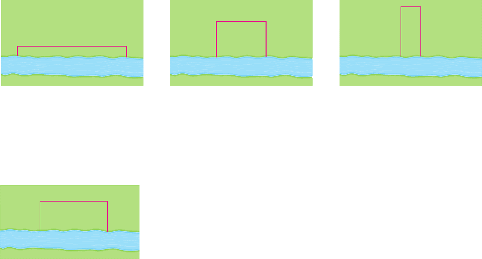
EXAMPLE 2 A cylindrical can is to be made to hold 1 L of oil. Find the dimensions

that will minimize the cost of the metal to manufacture the can.

SOLUTION Draw the diagram as in Figure 3, where is the radius and the height (both in

centimeters). In order to minimize the cost of the metal, we minimize the total surface

area of the cylinder (top, bottom, and sides). From Figure 4 we see that the sides are

made from a rectangular sheet with dimensions and h. So the surface area is

To eliminate we use the fact that the volume is given as 1 L, which we take to be

1000 cm . Thus

which gives . Substitution of this into the expression for gives

Therefore the function that we want to minimize is

To ﬁnd the critical numbers, we differentiate:

Then when , so the only critical number is .

Since the domain of is , we can’t use the argument of Example 1 concerning

endpoints. But we can observe that for and for

, so is decreasing for all to the left of the critical number and increas-

ing for all to the right. Thus must give rise to an absolute minimum.

[Alternatively, we could argue that as and as , so

there must be a minimum value of , which must occur at the critical number. See

Figure 5.]

The value of corresponding to is

h !

1000

)

1000

)

"500!

)

2!3

! 2

500

)

! 2r

r !

500!

)

A"r#

r l "A"r# l "r l 0

A"r# l "

r !

500!

)

rAr $

500!

)

A&"r# $ 0r

500!

)

A&"r#

"0, "#A

r !

500!

)

! 500A&"r# ! 0

A&"r# ! 4

)

r !

2000

)

! 500#

r $ 0A"r# ! 2

)

2000

A ! 2

)

' 2

)

1000

)

(

! 2

)

2000

Ah ! 1000!"

)

h ! 1000

A ! 2

)

' 2

)

x ! 600

AxA+"x# ! !4

A"600# ! 720,000

A"1200# ! 0A"0# ! 0, A"600# ! 720,000

Ax ! 600

2400 ! 4x ! 0

A&"x# ! 2400 ! 4x

258

|| ||

CHAPTER 4 APPLICATIONS OF DIFFERENTIATION

FIG URE 3

Area 2{πr@}

FIG URE 4

Area (2πr)h

2πr

1000

y=A(r)

FIG URE 5

N In the Applied Project on page 268 we investi-

gate the most economical shape for a can by

taking into account other manufacturing costs.

Thus, to minimize the cost of the can, the radius should be cm and the height

should be equal to twice the radius, namely, the diameter. M

The argument used in Example 2 to justify the absolute minimum is a variant

of the First Derivative Test (which applies only to local maximum or minimum values) and

is stated here for future reference.

FIRST DERIVATIVE TEST FOR ABSOLUTE EXTREME VALUES Suppose that is a criti-

cal number of a continuous function deﬁned on an interval.

(a) If for all and for all , then is the absolute

maximum value of .

(b) If for all and for all , then is the absolute

minimum value of .

An alternative method for solving optimization problems is to use implicit dif-

ferentiation. Let’s look at Example 2 again to illustrate the method. We work with the same

equations

but instead of eliminating h, we differentiate both equations implicitly with respect to r:

The minimum occurs at a critical number, so we set , simplify, and arrive at the

equations

and subtraction gives , or .

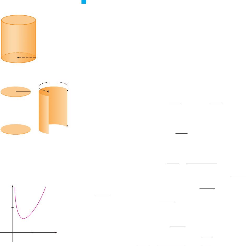
EXAMPLE 3 Find the point on the parabola that is closest to the point .

SOLUTION The distance between the point and the point is

(See Figure 6.) But if lies on the parabola, then , so the expression for

becomes

(Alternatively, we could have substituted to get in terms of alone.) Instead

of minimizing , we minimize its square:

(You should convince yourself that the minimum of occurs at the same point as the

minimum of , but is easier to work with.) Differentiating, we obtain

so when . Observe that when and when

, so by the First Derivative Test for Absolute Extreme Values, the absolute mini-y $ 2

f &"y# $ 0y

2f &"y#

0y ! 2f &"y# ! 0

f &"y# ! 2

(

! 1

)

y ' 2"y ! 4# ! y

! 8

! f "y# !

(

! 1

)

' "y ! 4#

xdy !

d !

(

! 1

)

' "y ! 4#

dx !

"x, y#

d !

"x ! 1#

' "y ! 4#

"x, y#"1, 4#

"1, 4#y

! 2x

h ! 2r2r ! h ! 0

2h ' rh& ! 02r ' h ' rh& ! 0

A& ! 0

)

rh '

)

h& ! 0A& ! 4

)

r ' 2

)

h ' 2

)

rh&

)

h ! 100A ! 2

)

' 2

)

NOTE 2

f "c#x $ cf &"x# $ 0x

cf &"x#

f "c#x $ cf &"x#

cf &"x# $ 0

NOTE 1

500!

)

SECTION 4.7 OPTIMIZATION PROBLEMS

|| ||

259

Module 4.7 takes you through six

additional optimization problems, including

animations of the physical situations.

TE C

2 3 4

¥=2x

(1,4)

(x,y)

FIG URE 6

mum occurs when . (Or we could simply say that because of the geometric nature

of the problem, it’s obvious that there is a closest point but not a farthest point.) The

corresponding value of is . Thus the point on closest to

is . M

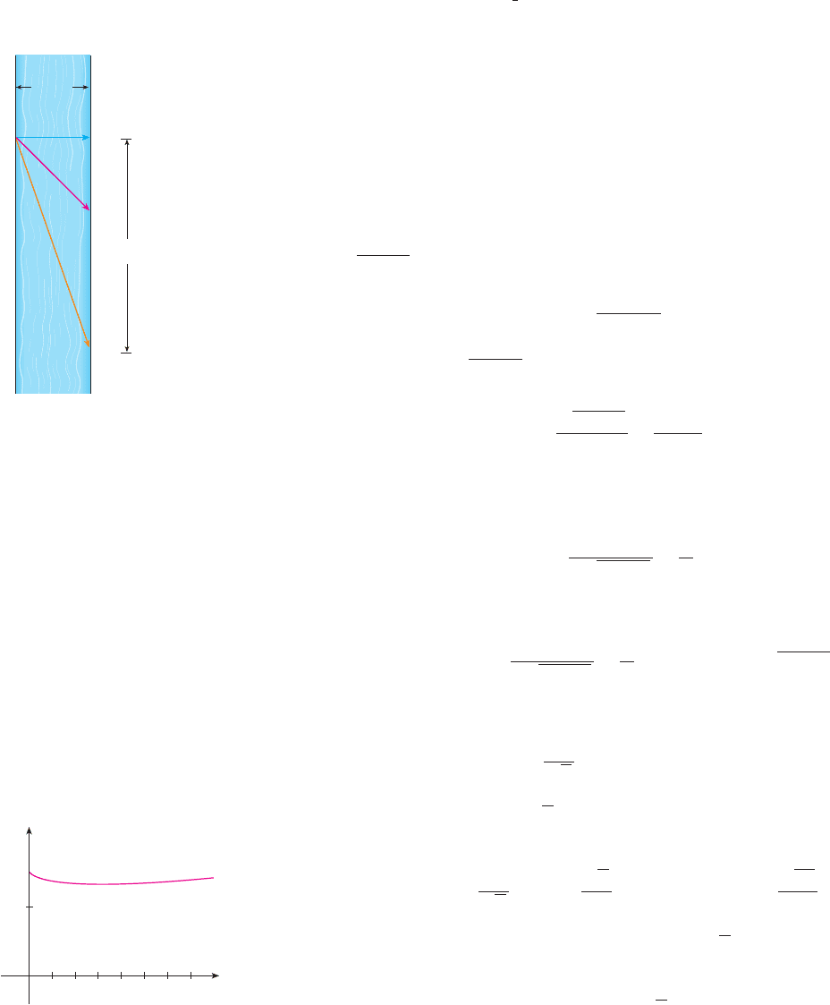
EXAMPLE 4 A man launches his boat from point on a bank of a straight river, 3 km

wide, and wants to reach point , 8 km downstream on the opposite bank, as quickly as

possible (see Figure 7). He could row his boat directly across the river to point and

then run to , or he could row directly to , or he could row to some point between

and and then run to . If he can row 6 km!h and run 8 km!h, where should he land to

reach as soon as possible? (We assume that the speed of the water is negligible com-

pared with the speed at which the man rows.)

SOLUTION If we let be the distance from to , then the running distance is

and the Pythagorean Theorem gives the rowing distance as

. We use the equation

Then the rowing time is and the running time is , so the total time

as a function of is

The domain of this function is . Notice that if , he rows to and if ,

he rows directly to . The derivative of is

Thus, using the fact that , we have

The only critical number is . To see whether the minimum occurs at this criti-

cal number or at an endpoint of the domain , we evaluate at all three points:

Since the smallest of these values of occurs when , the absolute minimum

value of must occur there. Figure 8 illustrates this calculation by showing the graph

of .

Thus the man should land the boat at a point km ( km) downstream from

his starting point.

)3.49!

x ! 9!

T"8# !

) 1.42 T

(

! 1 '

) 1.33T"0# ! 1.5

T$0, 8%

x ! 9!

x !

! 81&?16x

! 9"x

' 9#&?

4x ! 3

' 9

&?T&"x# ! 0

x % 0

T&"x# !

' 9

x ! 8Cx ! 0$0, 8%T

T"x# !

' 9

8 ! x

"8 ! x#!8

' 9

time !

distance

rate

' 9

! 8 ! x

DCx

CDBB

"2, 2#

"1, 4#y

! 2xx !

! 2x

y ! 2

260

|| ||

CHAPTER 4 APPLICATIONS OF DIFFERENTIATION

8 km

3 km

FIG URE 7

FIG URE 8

2 4 6

y=T(x)

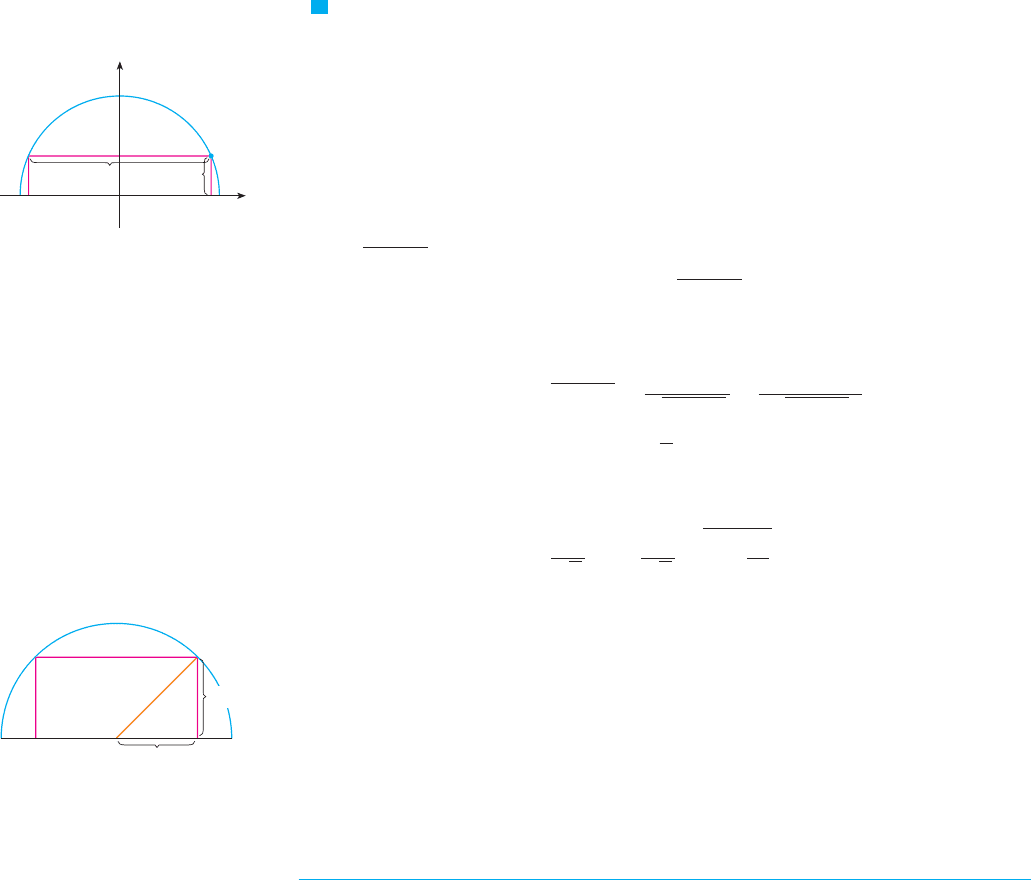
EXAMPLE 5 Find the area of the largest rectangle that can be inscribed in a semicircle

of radius .

SOLUTION 1 Let’s take the semicircle to be the upper half of the circle with

center the origin. Then the word inscribed means that the rectangle has two vertices on

the semicircle and two vertices on the -axis as shown in Figure 9.

Let be the vertex that lies in the ﬁrst quadrant. Then the rectangle has sides of

lengths and , so its area is

To eliminate we use the fact that lies on the circle and so

. Thus

The domain of this function is . Its derivative is

which is 0 when , that is, (since ). This value of gives a

maximum value of since and . Therefore the area of the largest

inscribed rectangle is

SOLUTION 2 A simpler solution is possible if we think of using an angle as a variable. Let

be the angle shown in Figure 10. Then the area of the rectangle is

We know that has a maximum value of 1 and it occurs when . So

has a maximum value of and it occurs when .

Notice that this trigonometric solution doesn’t involve differentiation. In fact, we

didn’t need to use calculus at all. M

APPLICATIONS TO BUSINESS AND ECONOMICS

In Section 3.7 we introduced the idea of marginal cost. Recall that if , the cost func-

tion, is the cost of producing units of a certain product, then the marginal cost is the rate

of change of with respect to . In other words, the marginal cost function is the deriva-

tive, , of the cost function.

Now let’s consider marketing. Let be the price per unit that the company can

charge if it sells units. Then is called the demand function (or price function) and we

would expect it to be a decreasing function of . If units are sold and the price per unit

is , then the total revenue is

and is called the revenue function. The derivative of the revenue function is called

the marginal revenue function and is the rate of change of revenue with respect to the

number of units sold.

R&R

R"x# ! xp"x#

p"x#

C&"x#

C"x#

)

!4r

)

!2sin 2

# ! "2r cos

#"r sin

# ! r

"2 sin

cos

# ! r

sin 2

(

! 2

! r

A"r# ! 0A"0# ! 0A

xx % 0x ! r!

! r

A& ! 2

! x

2"r

! 2x

! x

0 * x * r

A ! 2x

! x

y !

! x

' y

! r

"x, y#y

A ! 2xy

y2x

"x, y#

' y

! r

SECTION 4.7 OPTIMIZATION PROBLEMS

|| ||

261

(x,y)

_r r

FIG URE 9

r cos¨

rsin¨

FIG URE 10