Stewart J. Calculus

Подождите немного. Документ загружается.

The second situation arises when the function is determined from a scientiﬁc experi-

ment through instrument readings or collected data. There may be no formula for the func-

tion (see Example 5).

In both cases we need to ﬁnd approximate values of deﬁnite integrals. We already know

one such method. Recall that the deﬁnite integral is deﬁned as a limit of Riemann sums,

so any Riemann sum could be used as an approximation to the integral: If we divide

into subintervals of equal length , then we have

where is any point in the th subinterval . If is chosen to be the left endpoint

of the interval, then and we have

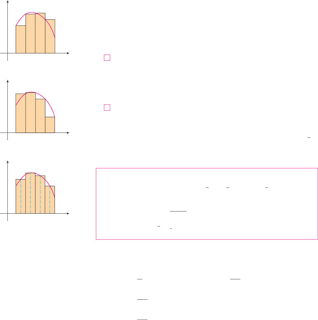
If , then the integral represents an area and (1) represents an approximation of this

area by the rectangles shown in Figure 1(a). If we choose to be the right endpoint, then

and we have

[See Figure 1(b).] The approximations and deﬁned by Equations 1 and 2 are called

the left endpoint approximation and right endpoint approximation, respectively.

In Section 5.2 we also considered the case where is chosen to be the midpoint of

the subinterval . Figure 1(c) shows the midpoint approximation , which appears

to be better than either or .

MIDPOINT RULE

and

Another approximation, called the Trapezoidal Rule, results from averaging the approx-

imations in Equations 1 and 2:

( f !x

" ! 2 f !x

" ! ( ( ( ! 2 f !x

n"1

" ! f !x

[

(

f !x

" ! f !x

)

(

f !x

" ! f !x

)

! ( ( ( !

(

f !x

n"1

" ! f !x

)

]

f !x" dx *

i!1

f !x

i"1

" 'x !

i!1

f !x

" 'x

i!1

(

f !x

i"1

" ! f !x

)

i"1

! x

" ! midpoint of (x

i"1

, x

)

'x !

b " a

where

f !x" dx * M

! 'x ( f !x

" ! f !x

" ! ( ( ( ! f !x

i"1

, x

)

f !x" dx * R

i!1

f !x

" 'x

! x

f !x" ) 0

f !x" dx * L

i!1

f !x

i"1

" 'x

! x

i"1

, x

)ix

f !x" dx *

i!1

f !x

" 'x

'x ! !b " a"%nn

(a, b)

532

|| ||

CHAPTER 8 TECHNIQUES OF INTEGRATION

⁄ ¤

– – ––

(a) Left endpoint approximation

x¸ ⁄ ¤ ‹ x¢

‹ x¢

(b) Right endpoint approximation

F I G U R E 1

TRAPEZOIDAL RULE

where and .

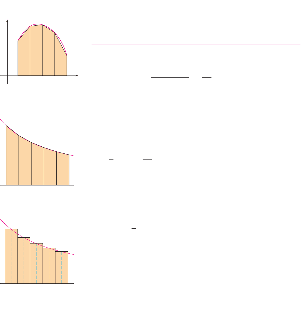
The reason for the name Trapezoidal Rule can be seen from Figure 2, which illustrates

the case . The area of the trapezoid that lies above the th subinterval is

and if we add the areas of all these trapezoids, we get the right side of the Trapezoidal

Rule.

EXAMPLE 1 Use (a) the Trapezoidal Rule and (b) the Midpoint Rule with to

approximate the integral .

SOLUTION

(a) With , and , we have , and so the Trape-

zoidal Rule gives

This approximation is illustrated in Figure 3.

(b) The midpoints of the ﬁve subintervals are , , , , and , so the Midpoint

Rule gives

This approximation is illustrated in Figure 4. M

In Example 1 we deliberately chose an integral whose value can be computed explicitly

so that we can see how accurate the Trapezoidal and Midpoint Rules are. By the Funda-

mental Theorem of Calculus,

The error in using an approximation is deﬁned to be the amount that needs to be added to

the approximation to make it exact. From the values in Example 1 we see that the errors

in the Trapezoidal and Midpoint Rule approximations for are

* 0.001239

and

* "0.002488

n ! 5

dx ! ln x

]

! ln 2 ! 0.693147 . . .

* 0.691908

1.1

1.3

1.5

1.7

1.9

dx * 'x ( f !1.1" ! f !1.3" ! f !1.5" ! f !1.7" ! f !1.9")

1.91.71.51.31.1

* 0.695635

! 0.1

1.2

1.4

1.6

1.8

dx * T

0.2

( f !1" ! 2 f !1.2" ! 2 f !1.4" ! 2 f !1.6" ! 2 f !1.8" ! f !2")

'x ! !2 " 1"%5 ! 0.2b ! 2n ! 5, a ! 1

!1%x" dx

n ! 5

f !x

i"1

" ! f !x

( f !x

i"1

" ! f !x

if !x" ) 0

! a ! i 'x'x ! !b " a"%n

f !x" dx * T

( f !x

" ! 2 f !x

" ! ( ( ( ! 2 f !x

n"1

" ! f !x

SECTION 8.7 APPROXIMATE INTEGRATION

|| ||

533

F I G U R E 3

x¸ ⁄ ¤ ‹ x¢

F I G U R E 2

Trapezoidal approximation

F I G U R E 4

1 2

f !x" dx ! approximation ! error

In general, we have

The following tables show the results of calculations similar to those in Example 1, but

for , and and for the left and right endpoint approximations as well as the

Trapezoidal and Midpoint Rules.

We can make several observations from these tables:

1. In all of the methods we get more accurate approximations when we increase the

value of . (But very large values of result in so many arithmetic operations that

we have to beware of accumulated round-off error.)

2. The errors in the left and right endpoint approximations are opposite in sign and

appear to decrease by a factor of about 2 when we double the value of .

3. The Trapezoidal and Midpoint Rules are much more accurate than the endpoint

approximations.

4. The errors in the Trapezoidal and Midpoint Rules are opposite in sign and appear

to decrease by a factor of about 4 when we double the value of .

5. The size of the error in the Midpoint Rule is about half the size of the error in the

Trapezoidal Rule.

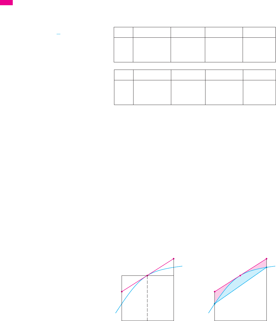
Figure 5 shows why we can usually expect the Midpoint Rule to be more accurate than

the Trapezoidal Rule. The area of a typical rectangle in the Midpoint Rule is the same as

the area of the trapezoid whose upper side is tangent to the graph at . The area of

this trapezoid is closer to the area under the graph than is the area of the trapezoid

used in the Trapezoidal Rule. [The midpoint error (shaded red) is smaller than the trape-

zoidal error (shaded blue).]

F I G U R E 5

i-1

ii-1

–

AQRD

PABCD

20n ! 5, 10

f !x" dx " M

andE

f !x" dx " T

534

|| ||

CHAPTER 8 TECHNIQUES OF INTEGRATION

5 0.745635 0.645635 0.695635 0.691908

10 0.718771 0.668771 0.693771 0.692835

20 0.705803 0.680803 0.693303 0.693069

5 "0.052488 0.047512 "0.002488 0.001239

10 "0.025624 0.024376 "0.000624 0.000312

20 "0.012656 0.012344 "0.000156 0.000078

Approximations to

Corresponding errors

N It turns out that these observations are true

in most cases.

Module 5.2 /8.7 allows you to

compare approximation methods.

TE C

These observations are corroborated in the following error estimates, which are proved

in books on numerical analysis. Notice that Observation 4 corresponds to the in each

denominator because . The fact that the estimates depend on the size of the

second derivative is not surprising if you look at Figure 5, because measures how

much the graph is curved. [Recall that measures how fast the slope of

changes.]

ERROR BOUNDS Suppose for . If and are the

errors in the Trapezoidal and Midpoint Rules, then

Let’s apply this error estimate to the Trapezoidal Rule approximation in Example 1. If

, then and . Since , we have , so

Therefore, taking , and in the error estimate (3), we see that

Comparing this error estimate of with the actual error of about , we see

that it can happen that the actual error is substantially less than the upper bound for the

error given by (3).

EXAMPLE 2 How large should we take in order to guarantee that the Trapezoidal

and Midpoint Rule approximations for are accurate to within ?

SOLUTION We saw in the preceding calculation that for , so we can

take , , and in (3). Accuracy to within means that the size of

the error should be less than . Therefore we choose so that

Solving the inequality for , we get

Thus will ensure the desired accuracy.n ! 41

n *

0.0006

* 40.8

12!0.0001"

2!1"

12n

0.0001

n0.0001

0.0001b ! 2a ! 1K ! 2

1 % x % 2

f ,!x"

% 2

0.0001

!1%x" dx

0.0024880.006667

2!2 " 1"

12!5"

150

* 0.006667

n ! 5K ! 2, a ! 1, b ! 2

f ,!x"

! 2

1%x % 11 % x % 2f ,!x" ! 2%x

f -!x" ! "1%x

f !x" ! 1%x

K!b " a"

24n

and

K!b " a"

12n

a % x % b

f ,!x"

% K

y ! f !x"f ,!x"

f ,!x"

!2n"

! 4n

SECTION 8.7 APPROXIMATE INTEGRATION

|| ||

535

N It’s quite possible that a lower value for

would sufﬁce, but is the smallest value for

which the error bound formula can

guarantee

accuracy to within .0.0001

N can be any number larger than all the

values of , but smaller values of

give better error bounds.

f ,!x"

For the same accuracy with the Midpoint Rule we choose so that

which gives

EXAMPLE 3

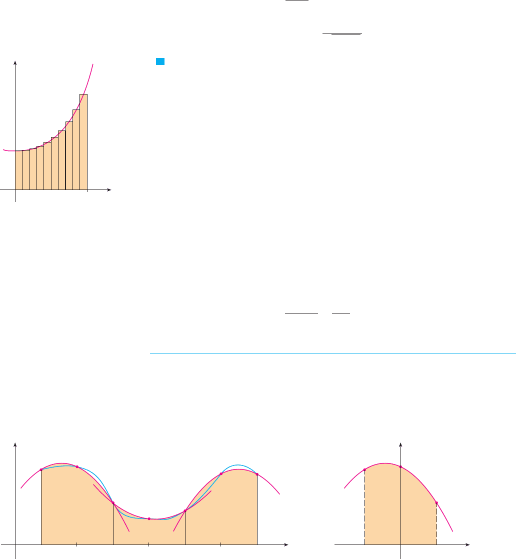
(a) Use the Midpoint Rule with to approximate the integral .

(b) Give an upper bound for the error involved in this approximation.

SOLUTION

(a) Since , and , the Midpoint Rule gives

Figure 6 illustrates this approximation.

(b) Since , we have and . Also, since

, we have and so

Taking , , , and in the error estimate (3), we see that an upper

bound for the error is

SIMPSON’S RULE

Another rule for approximate integration results from using parabolas instead of straight

line segments to approximate a curve. As before, we divide into subintervals of

equal length , but this time we assume that is an even number. Then

on each consecutive pair of intervals we approximate the curve by a parabola

as shown in Figure 7. If , then is the point on the curve lying above .

A typical parabola passes through three consecutive points , and .

a=x¸ ⁄ x™ x¢x£ xß=bx∞

P¸

P¡

P™

P¢

P£

Pß

P∞

F I G U R E 7

h_h

P¸(_h,y¸)

P¡(0,› )

P™(h,ﬁ)

F I G U R E 8

i!2

, P

i!1

, y

! f !x

y ! f !x" ) 0

nh ! 'x ! !b " a"%n

n(a, b)

6e!1"

24!10"

400

* 0.007

n ! 10b ! 1a ! 0K ! 6e

0 % f ,!x" ! !2 ! 4x

% 6e

% 10 % x % 1

f ,!x" ! !2 ! 4x

f -!x" ! 2xe

f !x" ! e

* 1.460393

! e

0.4225

! e

0.5625

! e

0.7225

! e

0.9025

)

! 0.1(e

0.0025

! e

0.0225

! e

0.0625

! e

0.1225

! e

0.2025

! e

0.3025

dx * 'x ( f !0.05" ! f !0.15" ! ( ( ( ! f !0.85" ! f !0.95")

n ! 10a ! 0, b ! 1

dxn ! 10

n *

0.0012

* 29

2!1"

24n

0.0001

536

|| ||

CHAPTER 8 TECHNIQUES OF INTEGRATION

F I G U R E 6

y=e

N Error estimates give upper bounds for

the error. They are theoretical, worst-case

scenarios. The actual error in this case turns

out to be about .0.0023

To simplify our calculations, we ﬁrst consider the case where , and

. (See Figure 8.) We know that the equation of the parabola through , and

is of the form and so the area under the parabola from to

But, since the parabola passes through , , and , we have

and therefore

Thus we can rewrite the area under the parabola as

Now, by shifting this parabola horizontally we do not change the area under it. This means

that the area under the parabola through , and from to in Figure 7

is still

Similarly, the area under the parabola through from to is

If we compute the areas under all the parabolas in this manner and add the results, we get

Although we have derived this approximation for the case in which , it is a rea-

sonable approximation for any continuous function and is called Simpson’s Rule after

the English mathematician Thomas Simpson (1710–1761). Note the pattern of coefﬁ-

cients: .1, 4, 2, 4, 2, 4, 2, . . . , 4, 2, 4, 1

f !x" ) 0

! 4y

! 2y

! 4y

! 2y

! ( ( ( ! 2y

n"2

! 4y

n"1

! y

! ( ( ( !

n"2

! 4y

n"1

! y

f !x" dx *

! 4y

! y

" !

! 4y

! y

! 4y

! y

x ! x

, P

, and P

! 4y

! y

x ! x

, P

! 4y

! y

! 4y

! y

! 2Ah

! 6C

! Ah

! Bh ! C

! C

! A!"h"

! B!"h" ! C ! Ah

" Bh ! C

!h, y

!0, y

!"h, y

! 2

! Ch

!2Ah

! 6C"

! 2

! Cx

!Ax

! Bx ! C" dx ! 2

!Ax

! C" dx

x ! h

x ! "hy ! Ax

! Bx ! C

, P

! h

! "h, x

! 0

SECTION 8.7 APPROXIMATE INTEGRATION

|| ||

537

N Here we have used Theorem 5.5.6.

Notice that is even and is odd.BxAx

! C

SIMPSON’S RULE

where is even and .

EXAMPLE 4 Use Simpson’s Rule with to approximate .

SOLUTION Putting , and in Simpson’s Rule, we obtain

Notice that, in Example 4, Simpson’s Rule gives us a much better approximation

to the true value of the integral than does the

Trapezoidal Rule or the Midpoint Rule . It turns out

(see Exercise 48) that the approximations in Simpson’s Rule are weighted averages of

those in the Trapezoidal and Midpoint Rules:

(

Recall that and usually have opposite signs and is about half the size of .

)

In many applications of calculus we need to evaluate an integral even if no explicit for-

mula is known for y as a function of x. A function may be given graphically or as a table

of values of collected data. If there is evidence that the values are not changing rapidly,

then the Trapezoidal Rule or Simpson’s Rule can still be used to ﬁnd an approximate value

for , the integral of y with respect to x.

EXAMPLE 5 Figure 9 shows data trafﬁc on the link from the United States to SWITCH,

the Swiss academic and research network, on February 10, 1998. is the data through-

put, measured in megabits per second . Use Simpson’s Rule to estimate the total

amount of data transmitted on the link up to noon on that day.

F I G U R E 9

3 6 9 12 15 18 21 24

t (hours)

!Mb"s#

D!t#

y dx

% 0.692835#!T

% 0.693771#

!ln 2 % 0.693147. . .#!S

% 0.693150#

% 0.693150

0.1

1.1

1.2

1.3

1.4

1.5

1.6

1.7

1.8

1.9

( f !1# ! 4 f !1.1# ! 2 f !1.2# ! 4 f !1.3# ! # # # ! 2 f !1.8# ! 4 f !1.9# ! f !2#)

dx % S

"x ! 0.1f !x# ! 1"x, n ! 10

!1"x# dxn ! 10

"x ! !b $ a#"nn

! 2 f !x

n$2

# ! 4 f !x

n$1

# ! f !x

f !x# dx % S

( f !x

# ! 4 f !x

# ! 2 f !x

# ! 4 f !x

# ! # # #

538

|| ||

CHAPTER 8 TECHNIQUES OF INTEGRATION

Thomas Simpson was a weaver who taught

himself mathematics and went on to become one

of the best English mathematicians of the 18th

century. What we call Simpson’s Rule was

actually known to Cavalieri and Gregory in the

17th century, but Simpson popularized it in his

best-selling calculus textbook,

A New Treatise

of Fluxions.

SI M PS O N

SOLUTION Because we want the units to be consistent and is measured in megabits

per second, we convert the units for from hours to seconds. If we let be the

amount of data (in megabits) transmitted by time , where is measured in seconds, then

. So, by the Net Change Theorem (see Section 5.4), the total amount of data

transmitted by noon (when ) is

We estimate the values of at hourly intervals from the graph and compile them in

the table.

Then we use Simpson’s Rule with and to estimate the integral:

Thus the total amount of data transmitted up to noon is about 144,000 megabits, or

144 gigabits. M

The table in the margin shows how Simpson’s Rule compares with the Midpoint Rule

for the integral , whose true value is about 0.69314718. The second table shows

how the error in Simpson’s Rule decreases by a factor of about 16 when is doubled.

(In Exercises 27 and 28 you are asked to verify this for two additional integrals.) That is

consistent with the appearance of in the denominator of the following error estimate for

Simpson’s Rule. It is similar to the estimates given in (3) for the Trapezoidal and Midpoint

Rules, but it uses the fourth derivative of .

ERROR BOUND FOR SIMPSON’S RULE Suppose that for

. If is the error involved in using Simpson’s Rule, then

K!b $ a#

180n

a % x % b

!4#

!x#

% K

!1"x# dx

! 143,880

! 2!1.1# ! 4!1.3# ! 2!2.8# ! 4!5.7# ! 2!7.1# ! 4!7.7# ! 7.9)

3600

(3.2 ! 4!2.7# ! 2!1.9# ! 4!1.7# ! 2!1.3# ! 4!1.0#

43,200

A!t# dt %

(D!0# ! 4D!3600# ! 2D!7200# ! # # # ! 4D!39,600# ! D!43,200#)

"t ! 3600n ! 12

D!t#

A!43,200# !

43,200

D!t# dt

t ! 12 & 60

! 43,200

A'!t# ! D!t#

A!t#t

D!t#

SECTION 8.7 APPROXIMATE INTEGRATION

|| ||

539

0 0 3.2 7 25,200 1.3

1 3,600 2.7 8 28,800 2.8

2 7,200 1.9 9 32,400 5.7

3 10,800 1.7 10 36,000 7.1

4 14,400 1.3 11 39,600 7.7

5 18,000 1.0 12 43,200 7.9

6 21,600 1.1

D!t#t !seconds#t !hours#D!t#t !seconds#t !hours#

4 0.69121989 0.69315453

8 0.69266055 0.69314765

16 0.69302521 0.69314721

4 0.00192729

8 0.00048663

16 0.00012197 $0.00000003

$0.00000047

$0.00000735

EXAMPLE 6 How large should we take in order to guarantee that the Simpson’s Rule

approximation for is accurate to within ?

SOLUTION If , then . Since , we have and so

Therefore we can take in (4). Thus, for an error less than , we should

choose so that

This gives

Therefore ( must be even) gives the desired accuracy. (Compare this with

Example 2, where we obtained for the Trapezoidal Rule and for the

Midpoint Rule.)

EXAMPLE 7

(a) Use Simpson’s Rule with to approximate the integral .

(b) Estimate the error involved in this approximation.

SOLUTION

(a) If , then and Simpson’s Rule gives

(b) The fourth derivative of is

and so, since , we have

Therefore, putting , and in (4), we see that the error is at

most

(Compare this with Example 3.) Thus, correct to three decimal places, we have

dx % 1.463

76e!1#

180!10#

% 0.000115

n ! 10K ! 76e, a ! 0, b ! 1

0 % f

!4#

!x# % !12 ! 48 ! 16#e

! 76e

0 % x % 1

!4#

!x# ! !12 ! 48x

! 16x

f !x# ! e

% 1.462681

! 4e

0.49

! 2e

0.64

! 4e

0.81

! e

)

0.1

! 4e

0.01

! 2e

0.04

! 4e

0.09

! 2e

0.16

! 4e

0.25

! 2e

0.36

dx %

( f !0# ! 4 f !0.1# ! 2 f !0.2# ! # # # ! 2 f !0.8# ! 4 f !0.9# ! f !1#)

"x ! 0.1n ! 10

dxn ! 10

n ! 29n ! 41

nn ! 8

n (

0.00075

% 6.04

(

180!0.0001#

24!1#

180n

)

0.0001

0.0001K ! 24

!4#

!x#

% 24

1"x % 1x * 1f

!4#

!x# ! 24"x

f !x# ! 1"x

0.0001x

!1"x# dx

540

|| ||

CHAPTER 8 TECHNIQUES OF INTEGRATION

N Many calculators and computer algebra sys-

tems have a built-in algorithm that computes an

approximation of a deﬁnite integral. Some of

these machines use Simpson’s Rule; others use

more sophisticated techniques such as

adaptive

numerical integration. This means that if a func-

tion ﬂuctuates much more on a certain part of

the interval than it does elsewhere, then that

part gets divided into more subintervals. This

strategy reduces the number of calculations

required to achieve a prescribed accuracy.

N Figure 10 illustrates the calculation in

Example 7. Notice that the parabolic arcs are

so close to the graph of that they are

practically indistinguishable from it.

y ! e

y=e

F I G U R E 1 0

SECTION 8.7 APPROXIMATE INTEGRATION

|| ||

541

(Round your answers to six decimal places.) Compare your

results to the actual value to determine the error in each

approximation.

5. , 6. ,

7–18 Use (a) the Trapezoidal Rule, (b) the Midpoint Rule, and

speciﬁed value of . (Round your answers to six decimal places.)

8. ,

10. ,

11. , 12. ,

13.

14. ,

15. , 16. ,

17. , 18. ,

19. (a) Find the approximations and for the integral

(b) Estimate the errors in the approximations of part (a).

tions and to the integral in part (a) are accurate to

within ?

20. (a) Find the approximations and for .

(b) Estimate the errors in the approximations of part (a).

tions and to the integral in part (a) are accurate to

within ?

21. (a) Find the approximations , , and for

and the corresponding errors , , and .

(b) Compare the actual errors in part (a) with the error esti-

mates given by (3) and (4).

tions , , and to the integral in part (a) are accurate

to within ?

22. How large should be to guarantee that the Simpson’s Rule

approximation to is accurate to within ?

23. The trouble with the error estimates is that it is often very

difﬁcult to compute four derivatives and obtain a good upper

bound for by hand. But computer algebra systems

!4#

!x#

CAS

0.00001x

0.00001

sin x dxS

0.0001

1"x

dxM

0.0001

cos !x

# dx

n ! 10

cos

x dxn ! 6

1 ! y

n ! 10

ln!x

! 2# dxn ! 8

cos x

n ! 10

dzn ! 8

sin t dt

n ! 8

1 !

dxn ! 8

1"2

sin!e

t"2

# dt

n ! 6

1 ! t

! t

n ! 10

ln x

1 ! x

n ! 4

1"2

sin!x

# dxn ! 8

1 ! x

n ! 6

dxn ! 8

sin x dx

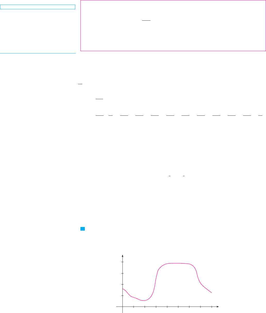
Let , where is the function whose graph is

shown.

(a) Use the graph to ﬁnd .

(b) Are these underestimates or overestimates of ?

(d) For any value of , list the numbers and

in increasing order.

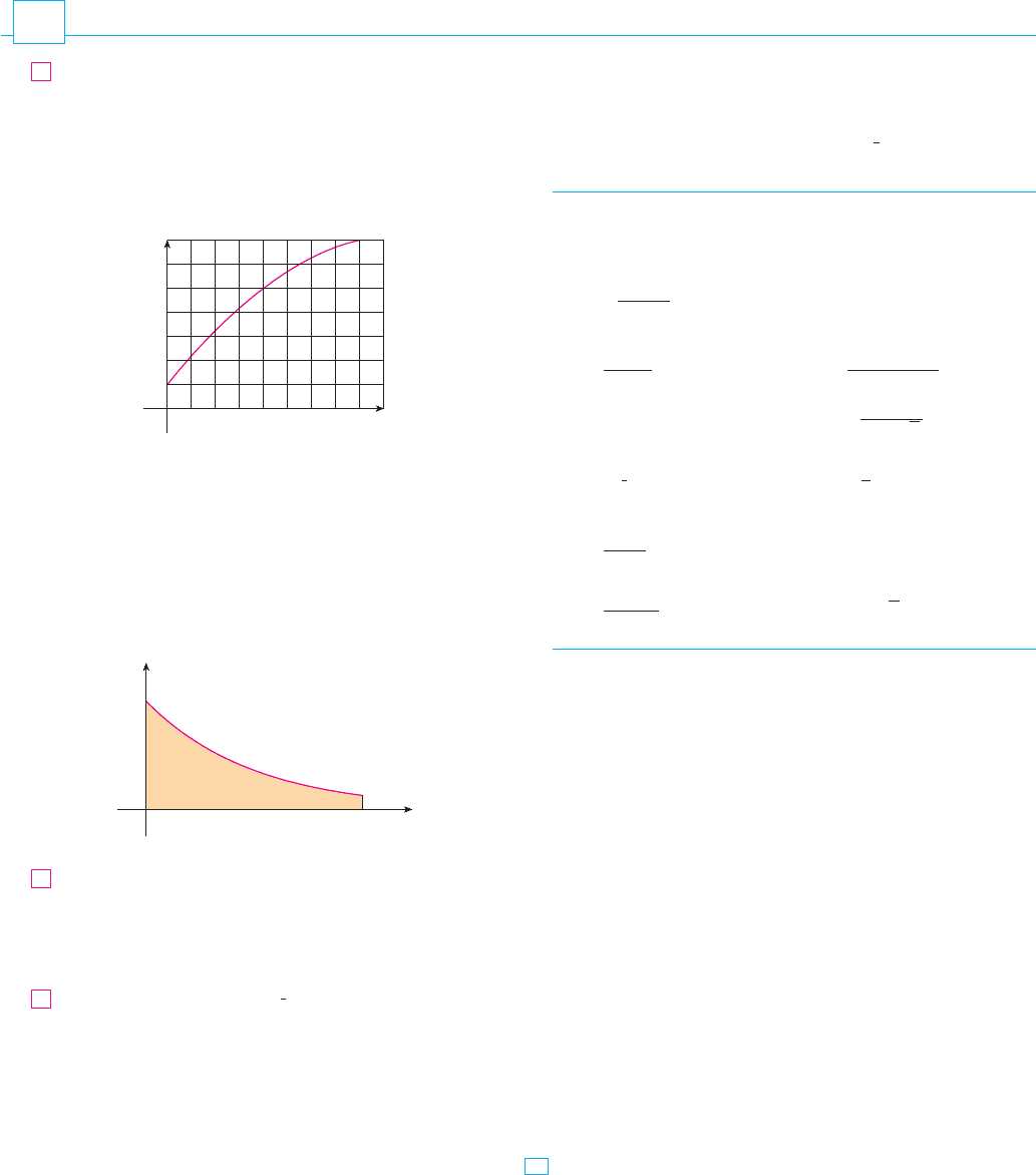
2. The left, right, Trapezoidal, and Midpoint Rule approxi-

mations were used to estimate , where is the

function whose graph is shown. The estimates were 0.7811,

0.8675, 0.8632, and 0.9540, and the same number of sub-

intervals were used in each case.

(a) Which rule produced which estimate?

(b) Between which two approximations does the true value of

lie?

;

Estimate using (a) the Trapezoidal Rule and

(b) the Midpoint Rule, each with . From a graph of the

integrand, decide whether your answers are underestimates or

overestimates. What can you conclude about the true value of

the integral?

;

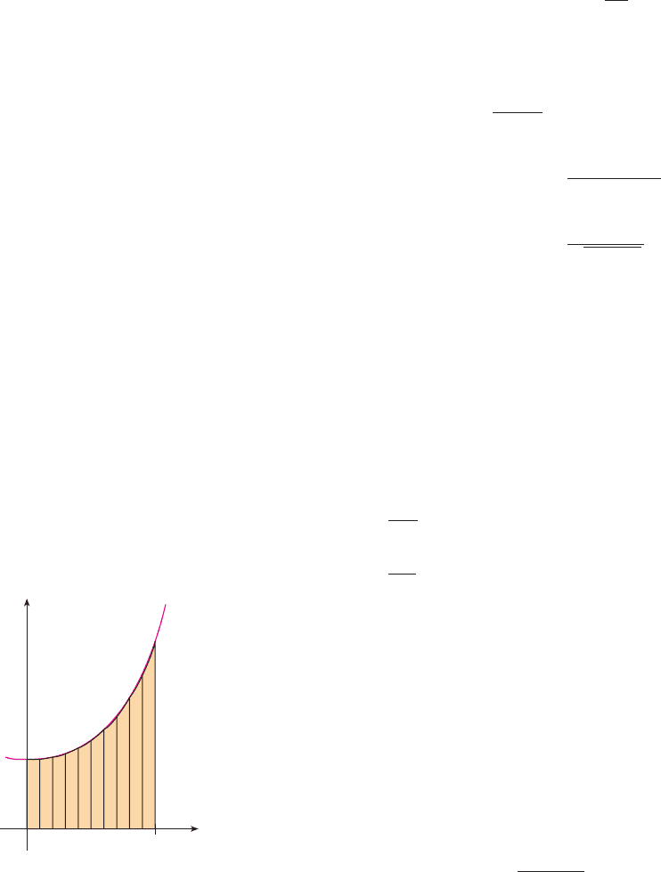
Draw the graph of in the viewing rectangle

by and let .

(a) Use the graph to decide whether , and under-

estimate or overestimate .

(b) For any value of , list the numbers and

in increasing order.

you think gives the best estimate of ?

5–6 Use (a) the Midpoint Rule and (b) Simpson’s Rule to

approximate the given integral with the speciﬁed value of . n

, R

, M

, and T

, R

, M

, T

, R

, M

I ! x

f !x# dx(0, 0.5)(0, 1)

f !x# ! sin

(

)

n ! 4

cos!x

y=ƒ

f !x# dx

2 3 4

, R

, M

, T

, R

, and M

fI ! x

f !x# dx

E X E R C I S E S

8.7