Townsend C.R., Begon M., Harper J.L. Essentials of Ecology

Подождите немного. Документ загружается.

matter of weeks), or from the change in climate at the end of the last ice age to

the present day and beyond (around 14,000 years and still counting). Migration

may be studied in butterﬂies over the course of days, or in the forest trees that are

still (slowly) migrating into deglaciated areas following that last ice age.

Although it is undoubtedly the case that ‘appropriate’ time scales vary, it is also

true that many ecological studies are not as long as they might be. Longer studies

cost more and require greater dedication and stamina. An impatient scientiﬁc

community, and the requirement for concrete evidence of activity for career pro-

gression, both put pressure on ecologists, and all scientists, to publish their work

sooner rather than later. Why are long-term studies potentially of such value? The

reduction over a few years in the numbers of a particular species of wild ﬂower,

or bird, or butterﬂy might be a cause for conservation concern – but one or more

decades of study may be needed to be sure that the decline is more than just an

expression of the random ups and downs of ‘normal’ population dynamics.

Similarly, a 2-year rise in the abundance of a wild rodent followed by a 2-year fall

might be part of a regular ‘cycle’ in abundance, crying out for an explanation. But

ecologists could not be sure until perhaps 20 years of study has allowed them to

record four or ﬁve repeats of such a cycle.

This does not mean that all ecological studies need to last for 20 years – nor

that every time an ecological study is extended the answer changes. But it does

emphasize the great value to ecology of the small number of long-term investiga-

tions that have been carried out or are ongoing.

1.2.2 The diversity of ecological evidence

Ecological evidence comes from a variety of different sources. Ultimately, eco-

logists are interested in organisms in their natural environments (though for many

organisms, the environment which is ‘natural’ for them now is itself manmade).

Progress would be impossible, however, if ecological studies were limited to such

Chapter 1 Ecology and how to do it

the need for long-term studies

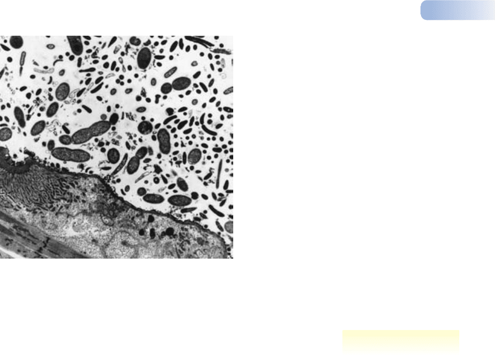
Figure 1.2

The diverse community of a termite’s gut. Termites can break

down lignin and cellulose from wood because of their mutualistic

relationships (see Section 8.4.4) with a diversity of microbes that

live in their guts.

AFTER BREZNAK, 1975

9781405156585_4_001.qxd 11/5/07 14:40 Page 9

natural environments. And, even in natural habitats, unnatural acts (experimental

manipulations) are often necessary in the search for sound evidence.

Many ecological studies involve careful observation and monitoring, in the

natural environment, of the changing abundance of one or more species over time,

or over space, or both. In this way, ecologists may establish patterns; for example,

that red grouse (birds shot for ‘sport’) exhibit regular cycles in abundance peaking

every 4 or 5 years, or that vegetation can be mapped into a series of zones as we

move across a landscape of sand dunes. But scientists do not stop at this point

– the patterns require explanation. Careful analysis of the descriptive data may

suggest some plausible explanations. But establishing what causes the patterns may

well require manipulative ﬁeld experiments: ridding the red grouse of intestinal

worms, hypothesized to underlie the cycles, and checking if the cycles persist

(they do not: Hudson et al., 1998), or treating experimental areas on sand dunes

with fertilizer to see whether the changing pattern of vegetation itself reﬂects a

changing pattern of soil productivity.

Perhaps less obviously, ecologists also often need to turn to laboratory systems

and even mathematical models. These have played a crucial role in the develop-

ment of ecology, and they are certain to continue to do so. Field experiments

are almost inevitably costly and difﬁcult to carry out. Moreover, even if time

and expense were not issues, natural ﬁeld systems may simply be too complex

to allow us to tease apart the consequences of the many different processes that

may be going on. Are the intestinal worms actually capable of having an effect on

reproduction or mortality of individual grouse? Which of the many species of sand

dune plants are, in themselves, sensitive to changing levels of soil productivity

and which are relatively insensitive? Controlled, laboratory experiments are often

the best way to provide answers to speciﬁc questions that are key parts of an

overall explanation of the complex situation in the ﬁeld.

Of course, the complexity of natural ecological communities may simply

make it inappropriate for an ecologist to dive straight into them in search of

understanding. We may wish to explain the structure and dynamics of a particu-

lar community of 20 animal and plant species comprising various competitors,

predators, parasites and so on (relatively speaking, a community of remarkable

simplicity). But we have little hope of doing so unless we already have some basic

understanding of even simpler communities of just one predator and one prey

species, or two competitors, or (especially ambitious) two competitors that also

share a common predator. For this, it is usually most appropriate to construct,

for our own convenience, simple laboratory systems that can act as benchmarks

or jumping-off points in our search for understanding.

What is more, you have only to ask anyone who has tried to rear caterpillar

eggs, or take a cohort of shrub cuttings through to maturity, to discover that

even the simplest ecological communities may not be easy to maintain or keep

free of unwanted pathogens, predators or competitors. Nor is it necessarily

possible to construct precisely the particular, simple, artiﬁcial community that

interests you; nor to subject it to precisely the conditions or the perturbation of

interest. In many cases, therefore, there is much to be gained from the analysis

of mathematical models of ecological communities: constructed and manipulated

according to the ecologist’s design.

On the other hand, although a major aim of science is to simplify, and thereby

make it easier to understand the complexity of the real world, ultimately it is the

Part I Introduction

observations and ﬁeld

experiments

laboratory experiments

simple laboratory systems...

. . . and mathematical models

9781405156585_4_001.qxd 11/5/07 14:40 Page 10

real world that we are interested in. The worth of models and simple laboratory

experiments must always be judged in terms of the light they throw on the

working of more natural systems. They are a means to an end – never an end in

themselves. Like all scientists, ecologists need to ‘seek simplicity, but distrust it’

(Whitehead, 1953).

1.2.3 Statistics and scientiﬁc rigor

For a scientist to take offence at some popular phrase or saying is to invite

accusations of a lack of a sense of humor. But it is difﬁcult to remain calm when

phrases like ‘There are lies, damn lies and statistics’ or ‘You can prove anything

with statistics’ are used, by those who should know better, to justify continuing

to believe what they wish to believe, whatever the evidence to the contrary.

There is no doubt that statistics are sometimes mis-used to derive dubious con-

clusions from sets of data that actually suggest either something quite different

or perhaps nothing at all. But these are not grounds for mistrusting statistics in

general – rather for ensuring that people are educated in at least the principles

of scientiﬁc evidence and its statistical analysis, so as to protect them from those

who may seek to manipulate their opinions.

In fact, not only is it not true that you can prove anything with statistics, the

contrary is the case: you cannot prove anything with statistics – that is not what

statistics are for. Statistical analysis is essential, however, for attaching a level of

conﬁdence to conclusions that can be drawn; and ecology, like all science, is a

search not for statements that have been ‘proved to be true’ but for conclusions

in which we can be conﬁdent.

Indeed, what distinguishes science from other activities – what makes science

‘rigorous’ – is that it is based not on statements that are simply assertions, but

that it is based (i) on conclusions that are the results of investigations (as we

have seen, of a wide variety of types) carried out with the express purpose of

deriving those conclusions; and (b) even more important, on conclusions to which

a level of conﬁdence can be attached, measured on an agreed scale. These points

are elaborated in Boxes 1.2 and 1.3.

Statistical analyses are carried out after data have been collected, and they help

us to interpret those data. There is no really good science, however, without fore-

thought. Ecologists, like all scientists, must know what they are doing, and why

they are doing it, while they are doing it. This is entirely obvious at a general

level: nobody expects ecologists to be going about their work in some kind of

daze. But it is perhaps not so obvious that ecologists should know how they are

going to analyze their data, statistically, not only after they have collected it, not

only while they are collecting it, but even before they begin to collect it. Ecologists

must plan, so as to be conﬁdent that they have collected the right kind of data,

and a sufﬁcient amount of data, to address the questions they hope to answer.

Ecologists typically seek to draw conclusions about groups of organisms over-

all: what is the birth rate of the bears in Yellowstone Park? What is the density

of weeds in a wheat ﬁeld? What is the rate of nitrogen uptake of tree saplings

in a nursery? In doing so, we can only very rarely examine every individual in a

group, or in the entire sampling area, and we must therefore rely on what we

hope will be a representative sample from the group or habitat. Indeed, even if we

examined a whole group (we might examine every ﬁsh in a small pond, say),

Chapter 1 Ecology and how to do it

ecology: a search for

conclusions in which we can

be conﬁdent

ecologists must think ahead

ecology relies on representative

samples

9781405156585_4_001.qxd 11/5/07 14:40 Page 11

Part I Introduction

1.2 QUANTITATIVE ASPECTS

1.2 Quantitative aspects

P-values

The term that is most often used, at the end of a

statistical test, to measure the strength of conclusions

being drawn is a P-value, or probability level. It is

important to understand what P-values are. Imagine

we are interested in establishing whether high abund-

ances of a pest insect in summer are associated with

high temperatures the previous spring, and imagine

that the data we have to address this question con-

sist of summer insect abundances and mean spring

temperatures for each of a number of years. We may

reasonably hope that statistical analysis of our data

will allow us either to conclude, with a stated degree

of conﬁdence, that there is an association, or to con-

clude that there are no grounds for believing there

to be an association (Figure 1.3).

Null hypotheses

To carry out a statistical test we ﬁrst need a null hypo-

thesis, which simply means, in this case, that there is

no association: that is, no association between insect

abundance and temperature. The statistical test (stated

simply) then generates a probability (a P-value) of getting

a data set like ours if the null hypothesis is correct.

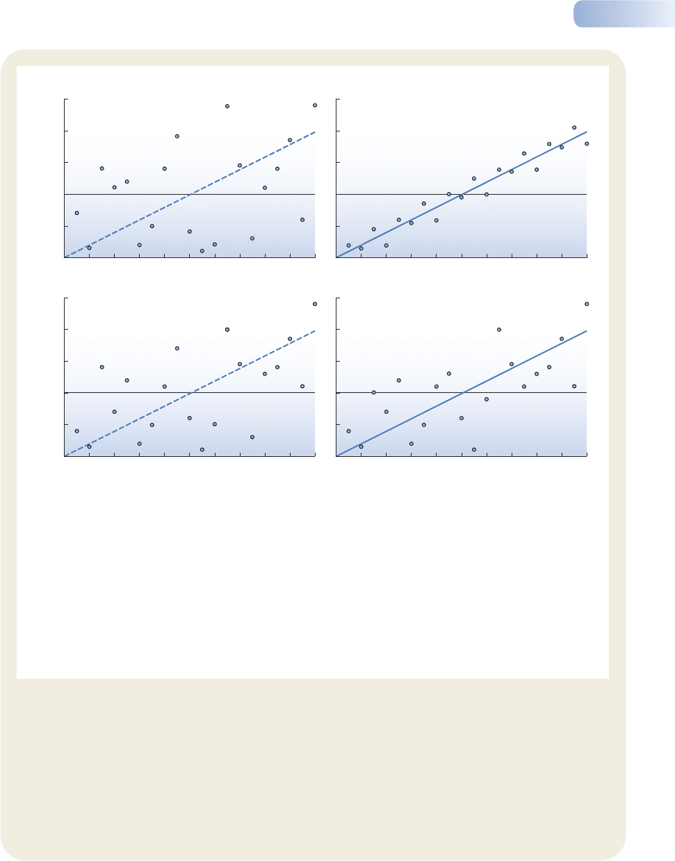
Suppose the data were like those in Figure 1.3a.

The probability generated by a test of association

on these data is P = 0.5 (equivalently 50%). This

means that, if the null hypothesis really was correct

(no association), then 50% of studies like ours should

generate just such a data set, or one even further from

the null hypothesis. So, if there was no association,

there would be nothing very remarkable in this data

set, and we could have no conﬁdence in any claim

that there was an association.

Suppose, however, that the data were like those in

Figure 1.3b, where the P-value generated is P = 0.001

(0.1%). This would mean that such a data set (or

one even further from the null hypothesis) could be

expected in only 0.1% of similar studies if there was

really no association. In other words, either something

very improbable has occurred, or there was an

association between insect abundance and spring

temperature. Thus, since by deﬁnition we do not expect

highly improbable events to occur, we can have a

high degree of conﬁdence in the claim that there was

an association between abundance and temperature.

Signiﬁcance testing

Both 50% and 0.01%, though, make things easy for us.

Where, between the two, do we draw the line? There

is no objective answer to this, and so scientists and

statisticians have established a convention in signiﬁc-

ance testing, which says that if P is less than 0.05

(5%), written P < 0.05 (e.g. Figure 1.3d), then results are

described as statistically signiﬁcant and conﬁdence can

be placed in the effect being examined (in our case, the

association between abundance and temperature),

whereas if P > 0.05, then there is no statistical founda-

tion for claiming the effect exists (e.g. Figure 1.3c).

A further elaboration of the convention often describes

results with P < 0.01 as ‘highly signiﬁcant’.

‘Insigniﬁcant’ results?

Naturally, some effects are strong (for example, there

is a powerful association between people’s weight

and their height) and others are weak (the association

between people’s weight and their risk of heart dis-

ease is real but weak, since weight is only one of

many important factors). More data are needed to

establish support for a weak effect than for a strong

one. A rather obvious but very important conclusion

follows from this: a P-value in an ecological study of

greater than 0.05 (lack of statistical signiﬁcance) may

mean one of two things:

1 There really is no effect of ecological importance.

2 The data are simply not good enough, or there

are not enough of them, to support the effect

even though it exists, possibly because the effect

itself is real but weak, and extensive data are

therefore needed but have not been collected.

Interpreting probabilities

9781405156585_4_001.qxd 11/5/07 14:40 Page 12

Chapter 1 Ecology and how to do it

shades of gray rather than the black and white of

‘proven effect’ and ‘no effect’. In particular, P-values

close to, but not less than, 0.05 suggest that some-

thing seems to be going on; they indicate, more than

anything else, that more data need to be collected so

that our conﬁdence in conclusions can be more

clearly established.

Throughout this book, then, studies of a wide

range of types are described, and their results often

10 11 12 13 14 15

10 11 12 13 14 15 10 11 12 13 14 15

10 11 12 13 14 15

(a) (b)

Abundance (numbers per m

)

Mean sprin

temperature (°C)

Figure 1.3

The results from four hypothetical studies of the relationship between insect pest abundance in summer and mean temperature the

previous spring. In each case, the points are the data actually collected. Horizontal lines represent the null hypothesis – that there is

no association between abundance and temperature, and thus the best estimate of expected insect abundance, irrespective of spring

temperature, is the mean insect abundance overall. The second line is the line of best ﬁt to the data, which in each case offers some

suggestion that abundance rises as temperature rises. However, whether we can be conﬁdent in concluding that abundance does rise

with temperature depends, as explained in the text, on statistical tests applied to the data sets. (a) The suggestion of a relationship is

weak (P = 0.5). There are no good grounds for concluding that the true relationship differs from that supposed by the null hypothesis

and no grounds for concluding that abundance is related to temperature. (b) The relationship is strong (P = 0.001) and we can be

conﬁdent in concluding that abundance increases with temperature. (c) The results are suggestive (P = 0.1) but it would not be

safe to conclude from them that abundance rises with temperature. (d) The results are not vastly different from those in (c) but

are powerful enough (P = 0.04, i.e. P < 0.05) for the conclusion that abundance rises with temperature to be considered safe.

Quoting P-values

Furthermore, applying the convention strictly and dog-

matically means that when P = 0.06 the conclusion

should be ‘no effect has been established’, whereas

when P = 0.04 the conclusion is ‘there is a signiﬁcant

effect’. Yet very little difference in the data is required

to move a P-value from 0.04 to 0.06. It is therefore far

better to quote exact P-values, especially when they

exceed 0.05, and think of conclusions in terms of

9781405156585_4_001.qxd 11/5/07 14:40 Page 13

Part I Introduction

have P-values attached to them. Of course, as this is

a textbook, the studies have been selected because

their results are signiﬁcant. Nonetheless, it is impor-

tant to bear in mind that the repeated statements

P < 0.05 and P < 0.01 mean that these are studies

where: (i) sufﬁcient data have been collected to

establish a conclusion in which we can be conﬁdent;

(ii) that conﬁdence has been established by agreed

means (statistical testing); and (iii) conﬁdence is being

measured on an agreed and interpretable scale.

Site A Site B Site A Site B

Mean number of seeds per plant

(b)(a)

1.3 QUANTITATIVE ASPECTS

1.3 Quantitative aspects

Standard errors and conﬁdence intervals

Following Box 1.2, another way in which the signiﬁc-

ance of results, and conﬁdence in them, is assessed

is through reference to standard errors. Again, simply

stated, statistical tests often allow standard errors to

be attached either to mean values calculated from a

set of observations or to slopes of lines like those in

Figure 1.3. Such mean values or slopes can, at best,

only ever be estimates of the ‘true’ mean value or true

slope, because they are calculated from data that

are only a sample of all the imaginable items of data

that could be collected. The standard error, then, sets

a band around the estimated mean (or slope, etc.)

within which the true mean can be expected to lie

with a given, stated probability. In particular, there is a

95% probability that the true mean lies within roughly

two standard errors (2 SE) of the estimated mean; we

call this the 95% conﬁdence interval.

Hence, when we have, say, two sets of observations,

each with its own mean value (for instance, the number

of seeds produced by plants from two sites, Figure 1.4)

the standard errors allow us to assess whether the

means are signiﬁcantly different from one another,

statistically. Roughly speaking, if each mean is more

than two standard errors from the other mean, then the

difference between them is statistically signiﬁcant with

P < 0.05. Thus, for the study illustrated in Figure 1.4a,

it would not be safe to conclude that plants from the

two sites differed in their seed production. However,

for the similar study illustrated in Figure 1.4b, the means

are roughly the same as they were in the ﬁrst study

and are roughly as far apart, but the standard errors

Attaching conﬁdence to results

Figure 1.4

The results of two hypothetical studies in which the

seed production of plants from two different sites

was compared. In all cases, the heights of the bars

represent the mean seed production of the sample of

plants examined, and the lines crossing those means

extend 1 SE above and below them. (a) Although the

means differ, the standard errors are relatively large

and it would not be safe to conclude that seed

production differed between the sites (P = 0.4).

(b) The differences between the means are very

similar to those in (a), but the standard errors

are much smaller, and it can be concluded with

conﬁdence that plants from the two sites differed

in their seed production (P < 0.05).

9781405156585_4_001.qxd 11/5/07 14:40 Page 14

we are likely to want to draw general conclusions from it: we might hope that

the ﬁsh in ‘our’ pond can tell us something about ﬁsh of that species in ponds

of that type, generally. In short, ecology relies on obtaining estimates from

representative samples. This is elaborated in Box 1.4.

Chapter 1 Ecology and how to do it

are smaller. Hence, the difference between the means

is signiﬁcant (P < 0.05), and we can conclude with

conﬁdence that plants from the two sites differed.

When are standard errors small?

Note that the large standard errors in the ﬁrst study,

and hence the lack of statistical signiﬁcance, could

have been due to data that were, for whatever reason,

more variable; but they may also have been due to

sampling fewer plants in the ﬁrst study than the

second. Standard errors are smaller, and statistical

signiﬁcance is easier to achieve, both when data

are more consistent (less variable) and when there

are more data.

1.4 QUANTITATIVE ASPECTS

1.4 Quantitative aspects

The discussion in Boxes 1.2 and 1.3 about when

standard errors will be small or large, or when our

conﬁdence in conclusions will be strong or weak, not

only has implications for the interpretation of data after

they have been collected, but also carries a general

message about planning the collection of data. In

undertaking a sampling program to collect data, the

aim is to satisfy a number of criteria:

1 That the estimate should be accurate or unbiased:

that is, neither systematically too high nor too low

as a result of some ﬂaw in the program.

2 That the estimate should have as narrow

conﬁdence limits (be as precise) as possible.

3 That the time, money and human effort invested

in the program should be used as effectively as

possible (because these are always limited).

Random and stratiﬁed random sampling

To understand these criteria, consider another hypo-

thetical example. Suppose that we are interested in

the density of a particular weed (say wild oat) in a

wheat ﬁeld. To prevent bias, it is necessary to ensure

that each part of the ﬁeld has an equal chance of

being selected for sampling. Sampling units should

therefore be selected at random. We might, for

example, divide the ﬁeld into a measured grid, pick

points on the grid at random, and count the wild

oat plants within a 50 cm radius of the selected grid

point. This unbiased method can be contrasted with

a plan to sample only weeds from between the rows

of wheat plants, giving too high an estimate, or within

the rows, giving too low an estimate (Figure 1.5a).

Remember, however, that random samples are not

taken as an end in themselves, but because random

sampling is a means to truly representative sampling.

Thus, randomly chosen sampling units may end up

being concentrated, by chance, in a particular part of

the ﬁeld that, unknown to us, is not representative of

the ﬁeld as a whole. It is often preferable, therefore, to

undertake stratiﬁed random sampling in which, in this

case, the ﬁeld is divided up into a number of equal-

sized parts (strata) and a random sample taken from

each. This way, the coverage of the whole ﬁeld is

more even, without our having introduced bias by

selecting particular spots for sampling.

Separating subgroups and directing effort

Suppose now, though, that half the ﬁeld is on a slope

facing southeast and the other half on a slope facing

Estimation: sampling, accuracy and precision

9781405156585_4_001.qxd 11/5/07 14:40 Page 15

Part I Introduction

southwest, and that we know that aspect (which way

the slope is facing) can affect weed density. Random

sampling (or stratiﬁed random sampling) ought still

to provide an unbiased estimate of density for the ﬁeld

as a whole, but for a given investment in effort, the

conﬁdence interval for the estimate will be unneces-

sarily high. To see why, consider Figure 1.5b. The

individual values from samples fall into two groups

a substantial distance apart on the density scale:

high from the southwest slope; low (mostly zero) from

the southeast slope. The estimated mean density is

close to the true mean (it is accurate), but the variation

among samples leads to a very large conﬁdence

interval (it is not very precise).

If, however, we acknowledge the difference between

the two slopes and treat them separately from the

outset, then we obtain means for each that have much

smaller conﬁdence intervals. What is more, if we

average those means and combine their conﬁdence

intervals to obtain an estimate for the ﬁeld as a whole,

then that interval too is much smaller than previously

(Figure 1.5b).

But has our effort been directed sensibly, with

equal numbers of samples from the southwest slope,

where there are lots of weeds, and the southeast

slope, where there are virtually none? The answer is

no. Remember that narrow conﬁdence intervals arise

from a combination of a large number of data points

and little intrinsic variability (see Box 1.3). Thus, if our

efforts had been directed mostly at sampling the

southwest slope, the increased amount of data would

have noticeably decreased the conﬁdence interval

(Figure 1.5c), whereas less sampling of the south-

east slope would have made very little difference to

that conﬁdence interval because of the low intrinsic

variability there. Careful direction of a sampling pro-

gram can clearly increase overall precision for a

given investment in effort. And generally, sampling

programs should, where possible, identify biologic-

ally distinct subgroups (males and females, old and

young, etc.) and treat them separately, but sample at

random within subgroups.

Random

sample

Individual

samples

Individual

samples

Between

rows only

Within

rows only

Study

Estimate

estimate

Combined

estimate

Combined

estimate

Weeds per m

Single study of

the whole field

SE and SW studied

separately, then combined

SW slopeSE slope

True mean True mean

SE and SW studied

separately, then combined

(a) (b)

(c)

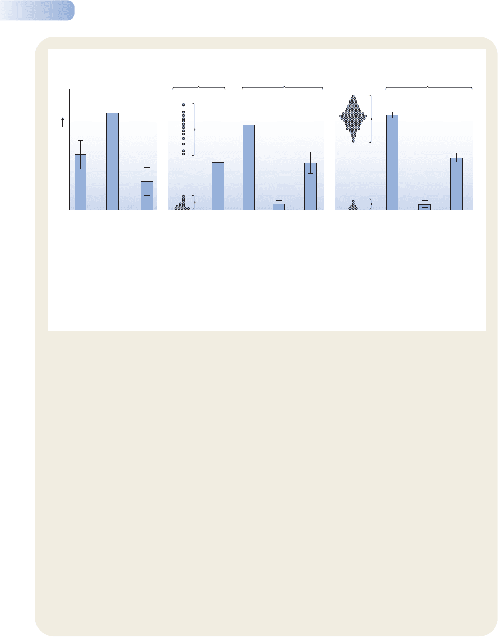
Figure 1.5

The results of hypothetical programs to estimate weed density in a wheat ﬁeld. (a) The three studies have equal precision (95%

conﬁdence intervals) but only the ﬁrst (from a random sample) is accurate. (b) In the ﬁrst study, individual samples from different

parts of the ﬁeld (southeast and southwest) fall into two groups (left); thus, the estimate, although accurate, is not precise (right).

In the second study, separate estimates for southeast and southwest are both accurate and precise – as is the estimate for the

whole ﬁeld obtained by combining them. (c) Following on from (b), most sampling effort is directed to the southwest, reducing the

conﬁdence interval there, but with little effect on the conﬁdence interval for the southeast. The overall interval is therefore reduced:

precision has been improved.

9781405156585_4_001.qxd 11/5/07 14:40 Page 16

1.3 Ecology in practice

In previous sections we have established in a general way how ecological under-

standing can be achieved, and how that understanding can be used to help us

predict, manage and control ecological systems. However, the practice of ecology

is easier said than done. To discover the real problems faced by ecologists and how

they try to solve them, it is best to consider some real research programs in a

little detail. While reading the following examples you should focus on how they

illuminate our three main points: (i) ecological phenomena occur at a variety

of scales; (ii) ecological evidence comes from a variety of different sources; and

(iii) ecology relies on truly scientiﬁc evidence and the application of statistics. Every

other chapter in this book will contain descriptions of similar studies, but in the

context of a systematic survey of the driving forces in ecology (Chapters 2–11) or

of the application of this knowledge to solve applied problems (Chapters 12–14).

For now, we content ourselves with seeking an appreciation of how four research

teams have gone about their business.

1.3.1 Brown trout in New Zealand: effects on

individuals, populations, communities and

ecosystems

It is rare for a study to encompass more than one or two of the four levels in

the biological hierarchy (individuals, populations, communities, ecosystems).

For most of the 20th century, physiological and behavioral ecologists (studying

individuals), population dynamicists, and community and ecosystem ecologists

tended to follow separate paths, asking different questions in different ways.

However, there can be little doubt that, ultimately, our understanding will be

enhanced considerably when the links between all these levels are made clear – a

point that can be illustrated by examining the impact of the introduction of an

exotic ﬁsh to streams in New Zealand.

Prized for the challenge they provide to anglers, brown trout (Salmo trutta)

have been transported from their native Europe all around the world; they were

introduced to New Zealand beginning in 1867, and self-sustaining populations

are now found in many streams, rivers and lakes there. Until quite recently, few

people cared about native New Zealand ﬁsh or invertebrates, so little information

is available on changes in the ecology of native species after the introduction

of trout. However, trout have colonized some streams but not others. We can

therefore learn a lot by comparing the current ecology of streams containing

trout with those occupied by non-migratory native ﬁsh in the genus Galaxias

(Figure 1.6).

Mayﬂy nymphs of various species commonly graze microscopic algae growing

on the beds of New Zealand streams, but there are some striking differences in

their activity rhythms depending on whether they are in Galaxias or trout

streams. In one experiment, nymphs collected from a trout stream and placed in

small artiﬁcial laboratory channels were less active during the day than the night,

whereas those collected from a Galaxias stream were active both day and night

(Figure 1.7a). In another experiment, with another mayﬂy species, records were

made of individuals visible in daylight on the surface of cobbles in artiﬁcial channels

Chapter 1 Ecology and how to do it

the individual level –

consequences for invertebrate

feeding behaviour

9781405156585_4_001.qxd 11/5/07 14:40 Page 17

placed in a real stream. Three treatments were each replicated three times – no

ﬁsh in the channels, trout present and Galaxias present. Daytime activity was

signiﬁcantly reduced in the presence of either ﬁsh species, but to a greater extent

when trout were present (Figure 1.7b).

These differences in activity pattern reﬂect the fact that trout rely prin-

cipally on vision to capture prey, whereas Galaxias rely on mechanical cues. Thus,

Part I Introduction

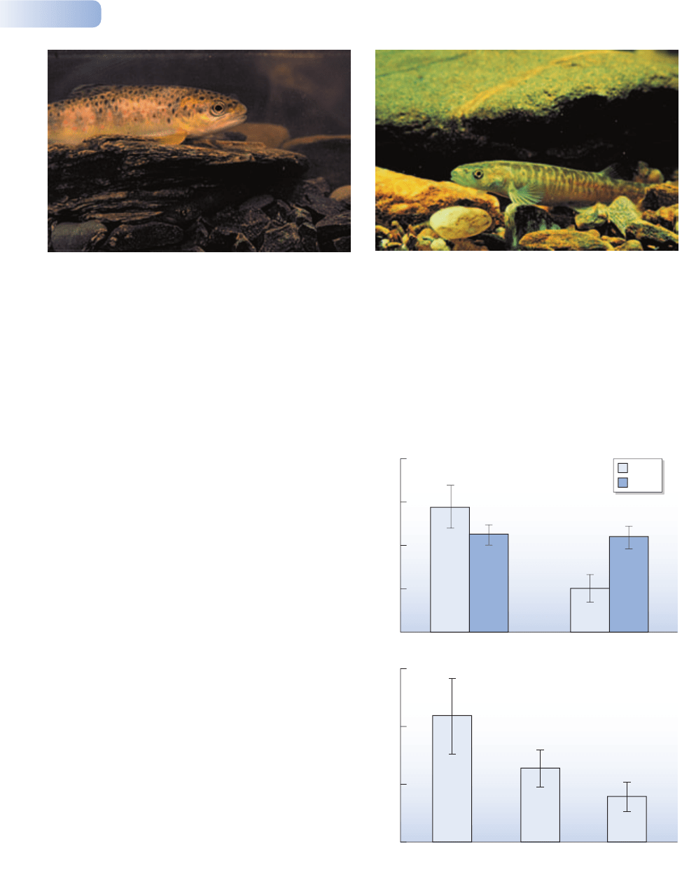
Figure 1.6

(a) A brown trout and (b) a Galaxias ﬁsh in a New Zealand stream – is the native Galaxias hiding from the introduced predator?

COURTESY OF ANGUS MCINTOSH

(a) (b)

Galaxias

Source stream

No fish

(a)

(b)

Night

Day

Trout streamGalaxias stream

Nesameletus visible

Deleatidium visible

Fish predation regime

Trout

Figure 1.7

(a) Mean number (± SE) of Nesameletus ornatus mayﬂy nymphs

collected either from a trout stream or a Galaxias stream that were

recorded by means of video as visible on the substrate surface

in laboratory stream channels during the day and night (in the

absence of ﬁsh). Mayﬂies from the trout stream are more nocturnal

than their counterparts from the Galaxias stream. (b) Mean number

(± SE) of Deleatidium mayﬂy nymphs observed on the upper

surfaces of cobbles during late afternoon in channels (placed in a real

stream) containing no ﬁsh, trout or Galaxias. The presence of a ﬁsh

discourages mayﬂies from emerging during the day, but trout have a

much stronger effect than Galaxias. In all cases, the standard errors

were sufﬁciently small for differences to be statistically signiﬁcant

(P < 0.05).

(a) AFTER MCINTOSH & TOWNSEND, 1994; (b) AFTER MCINTOSH & TOWNSEND, 1996

9781405156585_4_001.qxd 11/5/07 14:40 Page 18