Trauth M.H., MATLAB® Recipes for Earth Sciences, Third edition
Подождите немного. Документ загружается.

168 6 SIGNAL PROCESSING
and reverse ltering.
e functions
conv and filter that provide digital ltering in
MATLAB are best illustrated in terms of a simple running mean. e n ele-
ments of the vector x(t
1
), x(t
2
), x(t
3
), …, x(t
n
) are replaced by the arith-
metic means of subsets of the input vector. For instance, a running mean
over three elements computes the mean of inputs x(t
n–1
), x(t
n
), x(t
n+1
) to
obtain the output y(t
n
). We can illustrate this simply by generating a ran-
dom signal
clear
t = (1:100)';
randn('seed',0);
x1 = randn(100,1);
designing a lter that averages three data points of the input signal
b1 = [1 1 1]/3;
and convolving the input vector with the lter
y1 = conv(b1,x1);
e elements of b1 are the weights of the lter. In our example, all lter
weights are the same and equal to 1/3. Note that the
conv function yields a
vector that has the length n+m–1, where m is the length of the lter.
m1 = length(b1);
We can explore the contents of our workspace to check the length of the
input and output of
conv. Typing
whos
yields
Name Size Bytes Class Attributes
b1 1x3 24 double
m1 1x1 8 double
t 100x1 800 double
x1 100x1 800 double
y1 102x1 816 double
Here, we see that the actual input series x1 has a length of 100 data points,
whereas the output
y1 has two additional elements. Generally, convolution
introduces (m–1)/2 data points at each end of the data series. To compare
input and output signal, we clip the output signal at either end.

6.5 COMPARING FUNCTIONS FOR FILTERING DATA SERIES 169
6 SIGNAL PROCESSING
y1 = y1(2:101,1);
A more general way to correct the phase shi s of conv is
y1 = y1(1+(m1-1)/2:end-(m1-1)/2,1);
which, of course, only works for an odd number of lter weights. We can
then plot both input and output signals for comparison, using
legend to
display a legend for the plot.
plot(t,x1,'b-',t,y1,'r-')
legend('x1(t)','y1(t)')
is plot illustrates the e ect that the running mean has the original input
series. e output
y1 is signi cantly smoother than the input signal x1. If
we increase the length of the lter, we obtain an even smoother signal out-
put.
b2 = [1 1 1 1 1]/5;
m2 = length(b2);
y2 = conv(b2,x1);
y2 = y2(1+(m2-1)/2:end-(m2-1)/2,1);
plot(t,x1,'b-',t,y1,'r-',t,y2,'g-')
legend('x1(t)','y1(t)','y2(t)')
e next section provides a more general description of lters.
6.5 Comparing Functions for Filtering Data Series
e lters described in the previous section were very simple examples of
nonrecursive filters, in which the lter output y(t) depends only on the l-
ter input x(t) and the lter weights b
k
. Prior to introducing a more general
description of linear time-invariant lters, we replace the function
conv
by
filter, which can also be used for recursive filters. In this case, the
output y(t
n
) depends not only on the lter input x(t), but also on previous
elements of the output y(t
n–1
), y(t
n–2
), y(t
n–3
) and so on (Section 6.6). We
will rst use
conv for nonrecursive lters in order to compare the results of
conv and filter.
clear
t = (1:100)';
randn('seed',0);
x3 = randn(100,1);
170 6 SIGNAL PROCESSING
We design a lter that averages ve data points of the input signal.
b3 = [1 1 1 1 1]/5;
m3 = length(b3);
e input signal can be convolved using the function conv. As in the ex-
amples demonstrated in the previous section, the phase shi of
conv needs
to be corrected.
y3 = conv(b3,x3);
y3 = y3(1+(m3-1)/2:end-(m3-1)/2,1);
Next, we follow a similar procedure with the function filter and com-
pare the result with that obtained using the function
conv. In contrast to
the function
conv, the function filter yields an output vector with the
same length as the input vector; we also have to correct this output. Here,
the function
filter assumes that the lter is causal. e lter weights
are indexed n, n–1, n–2 and so on, and therefore no future elements of the
input vector, such as x(n+1), x(n+2) etc. are needed to compute the output
y(n). is is of great importance in electrical engineering, the classic eld
of MATLAB application, where lters are o en applied in real time. In
earth sciences, however, in most applications the entire signal is, in most
applications, available at the time of processing the data. e data series is
ltered by
y4 = filter(b3,1,x3);
and then the phase correction is carried out using
y4 = y4(1+(m3-1)/2:end-(m3-1)/2,1);
y4(end+1:end+m3-1,1) = zeros(m3-1,1);
which works only for an odd number of lter weights. is command sim-
ply shi s the output by
(m–1)/3 towards the lower end of the t-axis, and
then lls the data to the end with zeros. Comparing the ends of both out-
puts illustrates the e ect of this correction, where
y3(1:5,1)
y4(1:5,1)
yields
ans =
0.3734
0.4437
0.3044

6.5 COMPARING FUNCTIONS FOR FILTERING DATA SERIES 171
6 SIGNAL PROCESSING
0.4106
0.2971
ans =
0.3734
0.4437
0.3044
0.4106
0.2971
is was the lower end of the output. We can see that both vectors y3 and
y4 contain the same elements. Now we explorer the upper end of the data
vector, where
y3(end-5:end,1)
y4(end-5:end,1)
causes the output
ans =
0.2268
0.1592
0.3292
0.2110
0.3683
0.2414
ans =
0.2268
0.1592
0
0
0
0
e vectors are identical up to element y(end–m3+1), but then the second
vector
y4 contains zeros instead of true data values. Plotting the results
with
subplot(2,1,1), plot(t,x3,'b-',t,y3,'g-')
subplot(2,1,2), plot(t,x3,'b-',t,y4,'g-')
or in one single plot,
plot(t,x3,'b-',t,y3,'g-',t,y4,'r-')
shows that the results of conv and filter are identical except for the up-
per end of the data vector. ese observations are important for our next
steps in signal processing, particularly if we are interested in leads and lags
between various components of signals.
172 6 SIGNAL PROCESSING
b
i
T
+
T
a
i
+
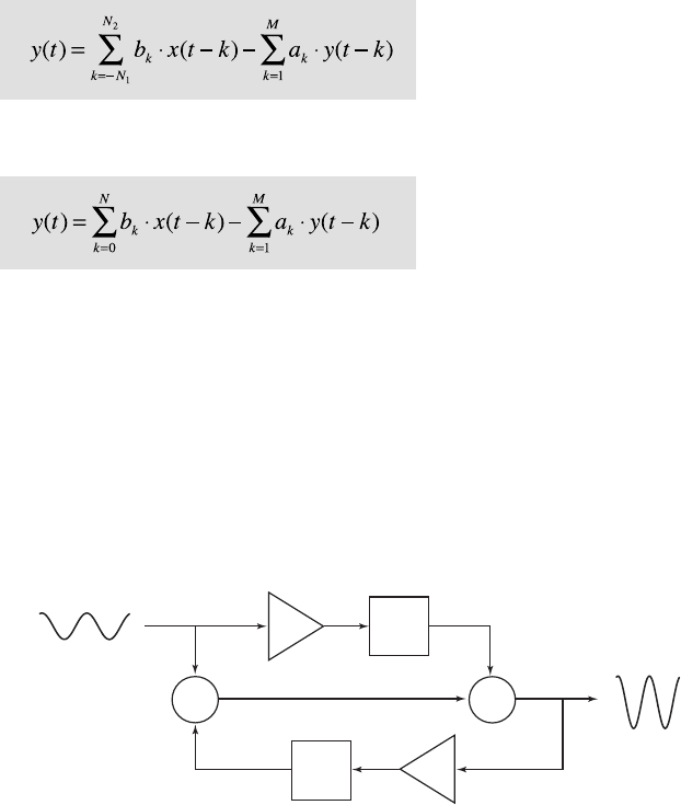
Input signal x(t)
Output signal y(t)
Fig. 6.2 Schematic of a linear time-invariant lter with an input x(t) and an output y(t). e
lter is characterized by its weights a
i
and b
i
. and the delay elements T. Nonrecursive lters
have only nonrecursive weights b
i
, whereas the recursive lter also requires the recursive
lter weights a
i
.
6.6 Recursive and Nonrecursive Filters
We now expand the nonrecursive lters by a recursive component, such that
the output y(t
n
) depends not only on the lter input x(t), but also on previ-
ous output values y(t
n–1
), y(t
n–2
), y(t
n–3
) and so on. is lter requires not
only the nonrecursive lter weights b
i
, but also the recursive lters weights
a
i
(Fig. 6.2), and can be described by the difference equation:
Although this is a non-causal version of the di erence equation, MATLAB
again uses the causal indexing,
with the known problems in the design of zero-phase lters. e larger of
the two quantities M, and N
1
+N
2
or N, is the order of the lter.
We use the same synthetic input signal as in the previous example to
illustrate the performance of a recursive lter.

6.7 IMPULSE RESPONSE 173
6 SIGNAL PROCESSING
clear
t = (1:100)';
randn('seed',0);
x5 = randn(100,1);
is input is then ltered using a recursive lter with a set of weights a5
and
b5,
b5 = [0.0048 0.0193 0.0289 0.0193 0.0048];
a5 = [1.0000 -2.3695 2.3140 -1.0547 0.1874];
m5 = length(b5);
y5 = filter(b5,a5,x5);
and the output corrected for the phase
y5 = y5(1+(m5-1)/2:end-(m5-1)/2,1);
y5(end+1:end+m5-1,1) = zeros(m5-1,1);
Now we can plot the results.
plot(t,x5,'b-',t,y5,'r-')
is lter clearly changes the signal dramatically. e output contains only
low-frequency components and all higher frequencies have been eliminated.
A comparison of the periodograms for the input and the output reveals that
all frequencies above f=0.1, corresponding to a period of τ =10 are sup-
pressed.
[Pxx,f] = periodogram(x5,[],128,1);
[Pyy,f] = periodogram(y5,[],128,1);
plot(f,Pxx,f,Pyy)
We have now designed a frequency-selective lter, i. e., a lter that elimi-
nates certain frequencies, while other periodicities remain relatively unaf-
fected. e next section introduces tools that are used to characterize a lter
in the time and frequency domains, and that help to predict the e ect of a
frequency-selective lter on arbitrary signals.
6.7 Impulse Response
e impulse response is a very convenient way of describing the character-
istics of a lter (Fig. 6.3). e impulse response h is useful in LTI systems
where the convolution of the input signal x(t) with h is used to obtain the
174 6 SIGNAL PROCESSING
0 5 10 15 20
0 5 10 15 20
−2
−1
0
1
2
−2
−1
0
1
2
t
t
x(t)
y(t)
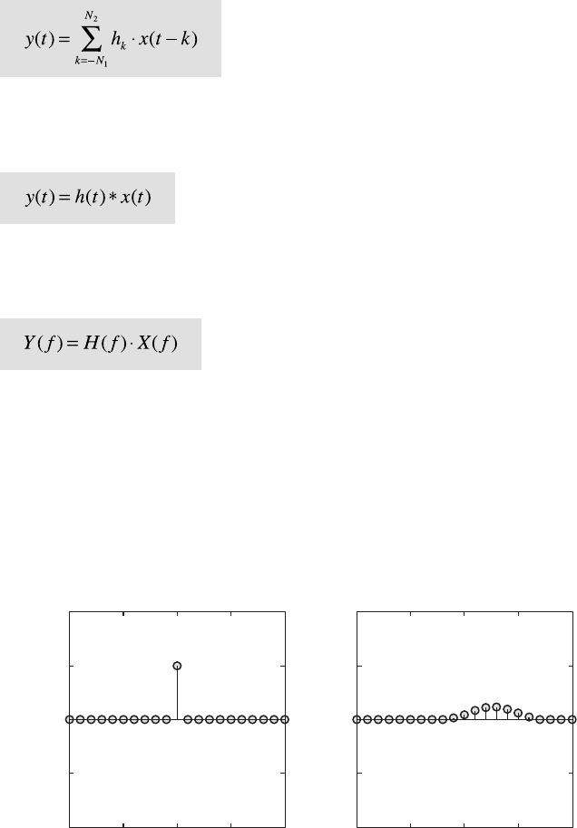
Unit Impulse Impulse Response
ab
Fig. 6.3 Transformation of a a unit impulse to compute b the impulse response of a system.
e impulse response is o en used to describe and predict the performance of a lter.
output signal y(t).
It can be shown that the impulse response h is identical to the lter weights
in nonrecursive lters, but not for recursive lters. e above convolution
equation is o en written in a short form:
In many examples, convolution in the time domain is replaced by a simple
multiplication of the Fourier transforms H(f ) and X(f ) in the frequency
domain.
e output signal y(t) in the time domain is then obtained by a reverse
Fourier transform of Y(f ). e signals are o en convolved in the frequency
domain rather than the time domain because of the relative simplicity of
the multiplication. However, the Fourier transformation itself introduces a
number of artifacts and distortions, and convolution in the frequency do-

6.7 IMPULSE RESPONSE 175
6 SIGNAL PROCESSING
main is therefore not without problems. In the following examples we apply
the convolution only in the time domain.
First, we generate a unit impulse:
clear
t = (0:20)';
x6 = [zeros(10,1);1;zeros(10,1)];
stem(t,x6), axis([0 20 -4 4])
e function stem plots the data sequence x6 as stems from the x-axis ter-
minated with circles for the data value. is might be a better way to plot
digital data than using the continuous lines generated by
plot. We now
feed this into the lter and explore the output. e impulse response is iden-
tical to the weights of nonrecursive lters.
b6 = [1 1 1 1 1]/5;
m6 = length(b6);
y6 = filter(b6,1,x6);
We again correct this for the phase shi of the function filter, although
this might not be important in this example.
y6 = y6(1+(m6-1)/2:end-(m6-1)/2,1);
y6(end+1:end+m6-1,1) = zeros(m6-1,1);
We obtain an output vector y6 of the same length and phase as the input
vector
x6. We now plot the results for comparison.
stem(t,x6)
hold on
stem(t,y6,'filled','r')
axis([0 20 -2 2])
hold off
In contrast to plot, the function stem accepts only one data series, and
the second series
y6 is therefore overlaid on the same plot using the func-
tion
hold. e e ect of the lter is clearly seen on the plot: it averages the
unit impulse over a length of ve elements. Furthermore, the values of the
output equal the lter weights of
a6, in our example 0.2 for all elements of
a6 and y6.
For a recursive lter, however, the output
y6 does not match with the
lter weights. Once again, an impulse is generated rst of all.
clear
176 6 SIGNAL PROCESSING
t = (0:20)';
x7 = [zeros(10,1);1;zeros(10,1)];
An arbitrary recursive lter with weights of a7 and b7 is then designed.
b7 = [0.0048 0.0193 0.0289 0.0193 0.0048];
a7 = [1.0000 -2.3695 2.3140 -1.0547 0.1874];
m7 = length(b7);
y7 = filter(b7,a7,x7);
y7 = y7(1+(m7-1)/2:end-(m7-1)/2,1);
y7(end+1:end+m7-1,1) = zeros(m7-1,1);
e stem plot of the input x2 and the output y2 shows an interesting im-
pulse response:
stem(t,x7)
hold on
stem(t,y7,'filled','r')
axis([0 20 -2 2])
hold off
e signal is smeared over a broader area, and is also shi ed towards the
right. is lter therefore not only a ects the amplitude of the signal, but
also shi s the signal towards lower or higher values. Such phase shi s are
usually unwanted characteristics of lters, although in some applications
shi s along the time axis might be of particular interest.
6.8 Frequency Response
We next investigate the frequency response of a lter, i. e., the e ect of a lter
on the amplitude and phase of a signal (Fig. 6.4). e frequency response
H(f ) of a lter is the Fourier transform of the impulse response h(f ). e
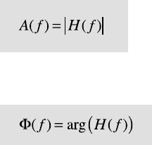
absolute value of the complex frequency response H( f ) is the magnitude
response of the lter A( f ).
e argument of the complex frequency response H(f ) is the phase response
of the lter.
6.8 FREQUENCY RESPONSE 177
6 SIGNAL PROCESSING
0.2
0.4
0.6
0.8
0 0.1 0.2 0.3 0.4
0 0.1 0.2 0.3 0.4
1
0
−1000
−800
−600
−400
−200
0
0.6
0.6
Frequency
Frequency
Magnitude
Phase in degrees
Magnitude
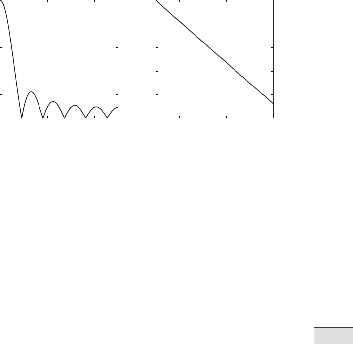
Unwrapped Phase
ab
Fig. 6.4 a Magnitude and b phase response of a running mean over eleven elements.
Since MATLAB lters are all causal it is di cult to explore the phase of
signals using the corresponding functions included in the Signal Processing
Toolbox. e user’s guide for this toolbox simply recommends that the lter
output be delayed in the time domain by a xed number of samples, as we
have done in the previous examples. As another example, a sine wave with a
period of 20 and an amplitude of 2 is used as an input signal.
clear
t = (1:100)';
x8 = 2*sin(2*pi*t/20);
A running mean over eleven elements is designed and this lter applied to
the input signal.
b8 = ones(1,11)/11;
m8 = length(b8);
y8 = filter(b8,1,x8);
e phase is corrected for causal indexing.
y8 = y8(1+(m8-1)/2:end-(m8-1)/2,1);
y8(end+1:end+m8-1,1) = zeros(m8-1,1);
Both input and output of the lter are plotted.