Trauth M.H., MATLAB® Recipes for Earth Sciences, Third edition

Подождите немного. Документ загружается.

208 7 SPATIAL DATA

plot(data(:,1),data(:,2),'o'), hold on

text(data(:,1)+1,data(:,2),labels), hold off

 is plot helps us to de ne the axis limits for gridding and contouring,

xlim = [420 470] and ylim = [70 120].  e function meshgrid trans-

forms the domain speci ed by vectors

x and y into arrays XI and YI.  e

rows of the output array

XI are copies of the vector x and the columns of the

output array

YI are copies of the vector y. We choose 1.0 as grid intervals.

x = 420:1:470; y = 70:1:120;

[XI,YI] = meshgrid(x,y);

 e biharmonic spline interpolation is used to interpolate the irregular-

spaced data at the grid points speci ed by

XI and YI.

ZI = griddata(data(:,1),data(:,2),data(:,3),XI,YI,'v4');

 e option v4 selects the biharmonic spline interpolation, which was the sole

gridding algorithm available until MATLAB4 was replaced by MATLAB5.

MATLAB provides various tools with which to display the results.  e sim-

plest way to display the gridding results is as a contour plot using

contour.

By default, the number of contour levels and the values of the contour levels

are chosen automatically.  e choice of the contour levels depends on the

minimum and maximum values of

contour(XI,YI,ZI)

Alternatively, the number of contours can be chosen manually, e. g., ten con-

tour levels.

contour(XI,YI,ZI,10)

Contouring can also be performed at values speci ed in a vector v. Since

the maximum and minimum values of

z are

min(data(:,3))

ans =

-27.4357

max(data(:,3))

ans =

21.3018

we choose

v = -40 : 10 : 20;

7.7 GRIDDING EXAMPLE 209

7 SPATIAL DATA

 e command

[c,h] = contour(XI,YI,ZI,v);

yields contour matrix c and a handle h that can be used as input to the func-

tion

clabel, which labels contours automatically.

clabel(c,h)

Alternatively, the plot can be labeled manually by selecting the manual op-

tion in the function

clabel.  is function places labels onto locations that

have been selected with the mouse. Labeling is terminated by pressing the

return key.

[c,h] = contour(XI,YI,ZI,v);

clabel(c,h,'manual')

Filled contours are an alternative to the empty contours used above.  is

function is used together with

colorbar which displays a legend for the

plot. In addition, we can plot the locations (small circles) and

z values (con-

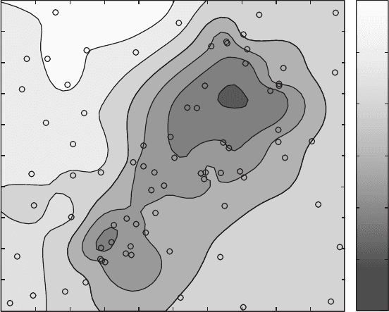
tour labels) of the true data points (Fig. 7.6).

contourf(XI,YI,ZI,v), colorbar, hold on

plot(data(:,1),data(:,2),'ko')

text(data(:,1)+1,data(:,2),labels), hold off

A pseudocolor plot is generated by using the function pcolor. Black con-

tours are also added at the same levels as in the above example.

pcolor(XI,YI,ZI), shading flat, hold on

contour(XI,YI,ZI,v,'k'), hold off

 e third dimension is added to the plot using the mesh command. We can

also use this example to introduce the function

view(az,el) to specify

the direction of viewing. Herein,

az is the azimuth or horizontal rotation

and

el is the elevation (both in degrees).  e values az = –37.5 and el = 30

de ne the default view for all 3D plots,

mesh(XI,YI,ZI), view(-37.5,30)

whereas az = 0 and el = 90 is directly overhead and the default 2D view

mesh(XI,YI,ZI), view(0,90)

 e function mesh provides one of many methods available in MATLAB

for 3D presentation, another commonly used function being

surf.  e

 gure may be rotated by selecting the Rotate 3D option on the Edit Tools

210 7 SPATIAL DATA

0.97

0.61

1.5

2.3

0.11

1.9

3.4

7.4

3.9

3.8

6.9

6.2

3.2

7.6

8.5

19 20

-6.5

-5.6

-3.6

-4.1

-5.2

-4.7

-8.5

-12

-9.5

-12

-10

-11

-8.1

-12

-8.7

-7.6

-7.5

-8.6

-10

-16

-14

-16

-13

-14

-15

-14

-16

-15

-13

-14

-16

-13

-14

-22

-21

-19

-21

-20

-22

-26

-27

-26

420 425 430 435 440 445 450 455 460 465 470

100

105

110

115

120

–40

–30

–20

–10

Fig. 7.6 Contour plot with the locations (small circles) and z-values (contour labels) of the

true data points.

menu. We also introduce the function colormap, which uses prede ned

color look-up tables for 3D graphs. Typing

help graph3d lists a number

of built-in colormaps, although colormaps can also be arbitrarily modi ed

and generated by the user. As an example, we use the colormap hot, which

is a black-red-yellow-white colormap.

surf(XI,YI,ZI), colormap('hot'), colorbar

Using Rotate 3D only rotates the 3D plot, not the colorbar.  e function

surfc combines both a surface and a 2D contour plot in one graph.

surfc(XI,YI,ZI)

 e function surfl can be used to illustrate an advanced application for

3D visualization, generating a 3D colored surface with interpolated shading

and lighting.  e axis labeling, ticks and background can be turned o by

typing

axis off. In addition, black 3D contours can be added to the sur-

face as above.  e grid resolution is increased prior to data plotting in order

to obtain smooth surfaces (Fig. 7.7).

7.8 COMPARISON OF METHODS AND POTENTIAL ARTIFACTS 211

7 SPATIAL DATA

Fig. 7.7  ree-dimensional colored surface with interpolated shading and simulated

lighting.  e axis labeling, ticks and background are turned o .  e plot also contains 3D

contours, in black.

[XI,YI] = meshgrid(420:0.25:470,70:0.25:120);

ZI = griddata(data(:,1),data(:,2),data(:,3),XI,YI,'v4');

surf(XI,YI,ZI), shading interp, light, axis off, hold on

contour3(XI,YI,ZI,v,'k'), hold off

 e biharmonic spline interpolation described in this section provides a so-

lution to most gridding problems. It was therefore, for some time, the only

gridding method that came with MATLAB. However, di erent applications

in earth sciences require di erent methods of interpolation, although they

all have their problems.  e next section compares biharmonic spline inter-

polation with other gridding methods and summarizes their strengths and

weaknesses.

7.8 Comparison of Methods and Potential Artifacts

 e  rst example in this section illustrates the use of the bilinear interpola-

tion technique for gridding irregular-spaced data. Bilinear interpolation is

an extension of the one-dimensional technique of linear interpolation in-

troduced in Section 5.5. In the two-dimensional case, linear interpolation

212 7 SPATIAL DATA

is  rst performed in one direction, and then in the other direction.  e

bilinear method would appear to be one of the simplest interpolation tech-

niques, which might intuitively not be expected to produce serious artifacts

or distortions in the data.  e opposite is true, however, as this method has

a number of disadvantages and other methods are therefore preferred in

many applications.

 e sample data used in the previous section can again be loaded to

study the e ects of a bilinear interpolation.

clear

data = load('normalfault.txt');

labels = num2str(data(:,3),2);

We now choose the option linear while using the function griddata to

interpolate the data.

[XI,YI] = meshgrid(420:0.25:470,70:0.25:120);

ZI = griddata(data(:,1),data(:,2),data(:,3),XI,YI,'linear');

 e results are plotted as contours.  e plot also includes the locations of

the control points.

v = -40 : 10 : 20;

contourf(XI,YI,ZI,v), colorbar, hold on

plot(data(:,1),data(:,2),'o'), hold off

 e new surface is restricted to the area that contains control points: by

default, bilinear interpolation does not extrapolate beyond this region.

Furthermore, the contours are rather angular compared to the smooth

shape of the contours from the biharmonic spline interpolation.  e most

important character of the bilinear gridding technique, however, is illus-

trated by a projection of the data in a vertical plane.

plot(XI,ZI,'k'), hold on

plot(data(:,1),data(:,3),'ro')

text(data(:,1)+1,data(:,3),labels)

title('Linear Interpolation'), hold off

 is plot shows the projection of the estimated surface (vertical lines) and

the labeled control points.  e z-values at the grid points never exceed the

z-values of the control points. As with the linear interpolation of time series

(Section 5.5), bilinear interpolation causes signi cant smoothing of the data

and a reduction in high-frequency variations.

Biharmonic spline interpolations are, in many ways, the other extreme.

 ey are o en used for extremely irregular-spaced and noisy data.

7.8 COMPARISON OF METHODS AND POTENTIAL ARTIFACTS 213

7 SPATIAL DATA

[XI,YI] = meshgrid(420:0.25:470,70:0.25:120);

ZI = griddata(data(:,1),data(:,2),data(:,3),XI,YI,'v4');

v = -40 : 10 : 20;

contourf(XI,YI,ZI,v), colorbar, hold on

plot(data(:,1),data(:,2),'o'), hold off

 e contours suggest an extremely smooth surface. In many applications,

this solution is very useful, but the method also produces a number of ar-

tifacts. As we can see from the next plot, the estimated values at the grid

points are o en beyond the range of the measured z-values.

plot(XI,ZI,'k'), hold on

plot(data(:,1),data(:,3),'o')

text(data(:,1)+1,data(:,3),labels)

title('Biharmonic Spline Interpolation'), hold off

 is can sometimes be appropriate and does not smooth the data in the way

that bilinear gridding does. However, introducing very close control points

with di erent z-values can cause serious artifacts. As an example, we intro-

duce one reference point with a z-value of +5 close to a reference point with

a negative z-value of around –26.

data(79,:) = [450 105 5];

labels = num2str(data(:,3),2);

ZI = griddata(data(:,1),data(:,2),data(:,3),XI,YI,'v4');

v = -40 : 10 : 20;

contourf(XI,YI,ZI,v), colorbar, hold on

plot(data(:,1),data(:,2),'ko')

text(data(:,1)+1,data(:,2),labels), hold off

 e extreme gradient at the location (450,105) results in a paired low and

high (Fig. 7.8). In such cases, it is recommended that one of the two control

points be deleted and the z-value of the remaining control point be replaced

by the arithmetic mean of both z-values.

Extrapolation beyond the area supported by control points is a common

feature of spline interpolation (see also Section 5.5). Extreme local trends

combined with large areas with no data o en result in unrealistic estimates.

To illustrate these edge e ects we eliminate all control points in the upper-

le corner.

[i,j] = find(data(:,1)<435 & data(:,2)>105);

data(i,:) = [];

labels = num2str(data(:,3),2);

plot(data(:,1),data(:,2),'ko'), hold on

text(data(:,1)+1,data(:,2),labels), hold off

214 7 SPATIAL DATA

420 425 430 435 440 445 450 455 460 465 470

100

105

110

115

120

–40

–30

–20

–10

0.97

0.61

1.5

2.3

0.11

1.9

3.4

7.4

3.9

3.8

6.9

6.2

3.2

7.6

8.5

19 20

-6.5

-5.6

-3.6

-4.1

-5.2

-4.7

-8.5

-12

-9.5

-12

-10

-11

-8.1

-12

-8.7

-7.6

-7.5

-8.6

-10

-16

-14

-16

-13

-14

-15

-14

-16

-15

-13

-14

-16

-13

-14

-22

-21

-19

-21

-20

-22

-26

-27

-26

Fig. 7.8 Contour plot of a data set gridded using a biharmonic spline interpolation. At the

location (450,105), very close control points with di erent

z values have been introduced.

Interpolation causes a paired low and high, which is a common artefact in spline

interpolation of noisy data.

We again employ the biharmonic spline interpolation technique.

[XI,YI] = meshgrid(420:0.25:470,70:0.25:120);

ZI = griddata(data(:,1),data(:,2),data(:,3),XI,YI,'v4');

v = -40 : 10 : 40;

contourf(XI,YI,ZI,v)

caxis([-40 40])

colorbar

hold on

plot(data(:,1),data(:,2),'ko')

text(data(:,1)+1,data(:,2),labels)

hold off

As can be seen from the plot, this method extrapolates the gradients beyond

the area with control points, up to the edge of the map (Fig. 7.9). Such an

e ect is particular undesirable when gridding closed data, such as percent-

ages, or data that have only positive values. In such cases, it is recommended

that the estimated

z values be replaced by NaN. For instance, we delete the

areas with

z values larger than 20, which are regarded as unrealistic values.

7.8 COMPARISON OF METHODS AND POTENTIAL ARTIFACTS 215

7 SPATIAL DATA

420 425 430 435 440 445 450 455 460 465 470

100

105

110

115

120

−40

−30

−20

−10

–20

–10

–20

Fig. 7.9 Contour plot of a data set gridded using a biharmonic spline interpolation. No

control points are available in the upper le corner.  e spline interpolation then beyond

the area with control points using gradients at the map edges resulting in unrealistic

estimates at the grid points.

 e resulting plot now contains a sector with no data.

ZID = ZI;

ZID(find(ZID > 20)) = NaN;

contourf(XI,YI,ZID,v)

caxis([-40 40])

colorbar

hold on

plot(data(:,1),data(:,2),'ko')

text(data(:,1)+1,data(:,2),labels)

hold off

Alternatively, we can eliminate a rectangular area with no data.

ZID = ZI;

ZID(131:201,1:71) = NaN;

contourf(XI,YI,ZID,v)

caxis([-40 40])

colorbar

hold on

216 7 SPATIAL DATA

plot(data(:,1),data(:,2),'ko')

text(data(:,1)+1,data(:,2),labels)

hold off

In some examples, the area with no control points is simply concealed by

placing a legend on this part of the map.

Another very useful MATLAB gridding method is splines with tension

by Wessel and Bercovici (1998).  e tsplines use biharmonic splines in ten-

sion t, where the parameter t can vary between 0 and 1. A value of t=0

corresponds to a standard cubic spline interpolation. Increasing t reduces

undesirable oscillations between data points, e. g., the paired lows and highs

observed in one of the previous examples.  e limiting situation t → 1 cor-

responds to linear interpolation.

7.9 Statistics of Point Distributions

 is section is about the statistical distribution of objects within an area,

which may help explain the relationship between these objects and proper-

ties of the area. For instance, the spatial concentration of hand-axes in an

archaeological site may suggest that a larger population of hominins lived in

that part of the area: the clustered occurrence of fossils may document en-

vironmental conditions that were favorable to those particular organisms;

the alignment of volcanoes may o en help in mapping tectonic structures

concealed beneath the surface.

 e rest of the section introduces methods for the statistical analysis of

point distributions. We  rst consider a test for a uniform spatial distribu-

tion of objects, followed by a test for a random spatial distribution. Finally, a

simple test for clustered distributions of objects is presented.

Test for Uniform Distribution

In order to illustrate the test for a uniform distribution we  rst need to com-

pute some synthetic data.  e function

rand computes uniformly-distrib-

uted pseudo-random numbers drawn from a uniform distribution within

the unit interval. We compute xy data using

rand and multiply the data by

ten to obtain data within the interval [0,10].

clear

rand('seed',0)

data = 10 * rand(100,2);

7.9 STATISTICS OF POINT DISTRIBUTIONS 217

7 SPATIAL DATA

012345678910

Fig. 7.10 Two-dimensional plot of a point distribution.  e distribution of objects in the

 eld is tested for uniform distribution using the χ2–test.  e

xy data are now organized in

25 classes that are subareas of the size 2-by-2.

We can use the χ

-test introduced in Section 3.8 to test the hypothesis that

the data have a uniform distribution.  e xy data are now organized in 25

classes that are square subareas of the dimension 2-by-2.  is de nition of

the classes ignores the rule of thumb that the number of classes should be

close to the square root of the number of observations (see Section 3.3). Our

choice of classes, however, does not result in empty classes, which should be

avoided when applying the χ

-test. Furthermore, 25 classes produce integer

values for the expected number of observations that are more easy to work

with. We display the data as blue circles in a plot of y versus x.  e rectan-

gular areas are outlined with red lines (Fig. 7.10).

plot(data(:,1),data(:,2),'o')

hold on

x = 0:10; y = ones(size(x));

for i = 1:4, plot(x,2*i*y,'r-'), end

for i = 1:4, plot(2*i*y,x,'r-'), end

hold off

A three-dimensional version of a histogram hist3 is used to display the