Trauth M.H., MATLAB® Recipes for Earth Sciences, Third edition

Подождите немного. Документ загружается.

218 7 SPATIAL DATA

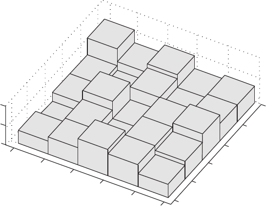
Fig. 7.11  ree-dimensional histogram displaying the numbers of objects for each subarea.

 e histogram was created using hist3.

spatial data organized in classes (Fig. 7.11).

hist3(data,[5 5]), view(30,70)

As with the equivalent two-dimensional function, the function hist3 can

be used to compute the frequency distribution

n_obs of the data.

n_obs = hist3(data,[5 5]);

n_obs = n_obs(:);

For a uniform distribution, the theoretical frequencies for the di erent

classes are identical.  e expected number of objects in each square area is

the size of the total area 10 × 10=100 divided by the 25 subareas or classes,

which comes to be four. To compare the theoretical frequency distribution

with the actual spatial distribution of objects, we generate a 5-by-5 array

with an identical number of four objects.

n_exp = 4 * ones(25,1);

 e χ

-test explores the squared di erences between the observed and ex-

7.9 STATISTICS OF POINT DISTRIBUTIONS 219

7 SPATIAL DATA

pected frequencies (Section 3.8).  e quantity χ

is de ned as the sum of the

squared di erences divided by the expected frequencies.

chi2_data = sum((n_obs - n_exp).^2 ./n_exp)

chi2 =

 e critical χ

can be calculated by using chi2inv.  e χ

-test requires the

degrees of freedom Φ. In our example, we test the hypothesis that the data

are uniformly distributed, i.e., we estimate only one parameter (Section 3.4).

 e number of degrees of freedom is therefore Φ=25–(1+1)=23. We test

the hypothesis at a p=95 % signi cance level.  e function

chi2inv com-

putes the inverse of the χ

CDF with parameters speci ed by Φ for the cor-

responding probabilities in p.

chi2_theo = chi2inv(0.95,25-1-1)

ans =

35.1725

Since the critical χ

of 35.1725 is well above the measured χ

of 14, we can-

not reject the null hypothesis and conclude that our data follow a uniform

distribution.

Test for Random Distribution

 e following example illustrates the test for random distribution of objects

within an area. We use the uniformly-distributed data generated in the pre-

vious example and display the point distribution.

clear

rand('seed',0)

data = 10 * rand(100,2);

plot(data(:,1),data(:,2),'o')

hold on

x = 0:10; y = ones(size(x));

for i = 1:9, plot(x,i*y,'r-'), end

for i = 1:9, plot(i*y,x,'r-'), end

hold off

We generate the three-dimensional histogram and use the function hist3

to count the objects per class. In contrast to the previous test, we now count

the subareas containing a certain number of observations.  e number of

subareas is larger than would usually be used for the previous test. In our

example, we use 49 subareas or classes.

220 7 SPATIAL DATA

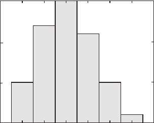
Frequency

Number of Objects

012345

Fig. 7.12 Frequency distribution of subareas with N objects. In our example, the subareas

with 0, …, 5 objects are counted.  e histogram of the frequency distribution is displayed

as a two-dimensional histogram using hist.

hist3(data,[7 7])

view(30,70)

counts = hist3(data,[7 7]);

counts = counts(:);

 e frequency distribution of those subareas that contain a speci c number

of objects follows a Poisson distribution (Section 3.4) if the objects are ran-

domly distributed. First, we compute a frequency distribution of the subar-

eas containing N objects. In our example, we count the subareas with 0, …,

5 objects. We also display the histogram of the frequency distribution as a

two-dimensional histogram using

hist (Fig. 7.12).

N = 0 : 5;

[n_obs,v] = hist(counts,N);

hist(counts,N)

title('Histogram')

xlabel('Number of observations N')

ylabel('Subareas with N observations')

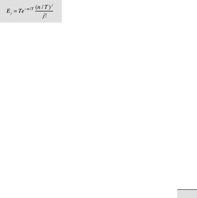
Here, the midpoints of the histogram intervals v correspond to the N=0, …, 5

objects contained in the subareas.  e expected number of subareas E

with

a certain number of objects j can be computed using

7.9 STATISTICS OF POINT DISTRIBUTIONS 221

7 SPATIAL DATA

where n is the total number of objects and T is the number of subareas. For

j=0, j! is taken to be 1. We compute the theoretical frequency distribution

using the equation shown above,

for i = 1 : 6

n_exp(i) = 49*exp(-100/49)*(100/49)^N(i)/factorial(N(i));

end

n_exp = sum(n_obs)*n_exp/sum(n_exp);

and display both the empirical and theoretical frequency distributions in a

single plot.

h1 = bar(v,n_obs);

hold on

h2 = bar(v,n_exp);

hold off

set(h1,'FaceColor','none','EdgeColor','r')

set(h2,'FaceColor','none','EdgeColor','b')

 e χ

-test is again employed to compare the empirical and theoretical dis-

tributions.  e test is performed at a p=95 % signi cance level. Since the

Poisson distribution is de ned by only one parameter (Section 3.4), the

number of degrees of freedom is Φ=6–(1+1)=4.  e measured χ

chi2 = sum((n_obs - n_exp).^2 ./n_exp)

chi2 =

1.4357

is well below the critical χ

, which is

chi2inv(0.95,6-1-1)

ans =

9.4877

We therefore cannot reject the null hypothesis and conclude that our data

follow a Poisson distribution and the point distribution is random.

Test for Clustering

Point distributions in geosciences are o en clustered. We use a nearest-

neighbor criterion to test a spatial distribution for clustering. Davis (2002)

222 7 SPATIAL DATA

published an excellent summary of the nearest-neighbor analysis, summa-

rizing the work of a number of other authors. Swan and Sandilands (1996)

presented a simpli ed description of this analysis.  e test for clustering

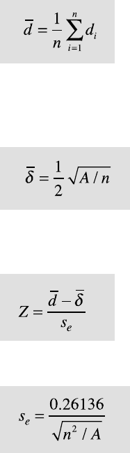
computes the distances d

separating all possible pairs of nearest points in

the  eld.  e observed mean nearest-neighbor distance is

where n is the total number of points or objects in the  eld.  e arithmetic

mean of all distances between possible pairs is related to the area covered

by the map.  is relationship is expressed by the expected mean nearest-

neighbor distance, which is

where A is the area covered by the map. Small values for this ratio then sug-

gest signi cant clustering, whereas large values indicate regularity or uni-

formity.  e test uses a Z statistic (Section 3.4), which is

where s

is the standard error of the mean nearest-neighbor distance, which

is de ned as

 e null hypothesis randomness is tested against two alternative hypotheses,

clustering and uniformity or regularity.  e Z statistic has critical values

of 1.96 and –1.96 at a signi cance level of 95 %. If –1.96<Z<+1.96, we cannot

reject the null hypothesis that the data are randomly distributed. If Z<–1.96,

we reject the null hypothesis and accept the  rst alternative hypothesis of

clustering. If Z>+1.96, we also reject the null hypothesis, but accept the sec-

ond alternative hypothesis of uniformity or regularity.

As an example, we again use the synthetic data analyzed in the previous

examples.

clear

7.9 STATISTICS OF POINT DISTRIBUTIONS 223

7 SPATIAL DATA

rand('seed',0)

data = 10 * rand(100,2);

plot(data(:,1),data(:,2),'o')

We  rst compute the pairwise Euclidian distance between all pairs of ob-

servations using the function

pdist (Section 9.4).  e resulting distance

matrix

distances is then converted into a symmetric, square format, so

that

distmatrix(i,j) denotes the distance between i and j objects in

the original data.

distances = pdist(data,'Euclidean');

distmatrix = squareform(distances);

 e following for loop  nds the nearest neighbors, stores the nearest-

neighbor distances and computes the mean distance.

for i = 1 : 100

distmatrix(i,i) = NaN;

k = find(distmatrix(i,:) == min(distmatrix(i,:)));

nearest(i) = distmatrix(i,k(1));

end

observednearest = mean(nearest)

observednearest =

0.5171

In our example, the mean nearest distance observednearest comes to

0.5471. Next, we calculate the area of the map.  e expected mean nearest-

neighbor distance is half the square root of the map area divided by the

number of observations.

maparea = (max(data(:,1)-min(data(:,1)))) ...

*(max(data(:,2)-min(data(:,2))));

expectednearest = 0.5 * sqrt(maparea/length(data))

expectednearest =

0.4940

In our example, the expected mean nearest-neighbor distance expected-

nearest is 0.4940. Finally, we compute the standard error of the mean

nearest-neighbor distance

se = 0.26136/sqrt(length(data).^2/maparea)

se =

0.0258

and the test statistic Z.

Z = (observednearest - expectednearest)/se

224 7 SPATIAL DATA

Z =

0.8960

In our example, Z is 0.8960. Since –1.96<Z<+1.96, we cannot reject the null

hypothesis and conclude that the data are randomly distributed, but not

clustered.

7.10 Analysis of Digital Elevation Models (by R. Gebbers)

Digital elevation models ( DEMs) and their derivatives (e. g., slope and as-

pect) can indicate surface processes such as lateral water  ow, solar irra-

diation or erosion.  e simplest derivatives of a DEM are the slope and the

aspect.  e slope (or gradient) is a measure of the steepness, the incline or

the grade of a surface measured in percentages or degrees.  e aspect (or

exposure) refers to the direction in which a slope faces.

We use the SRTM data set introduced in Section 7.5 to illustrate the

analysis of a digital elevation model for slope, aspect and other derivatives.

 e data are loaded by

clear

fid = fopen('S01E036.hgt','r');

SRTM = fread(fid,[1201,inf],'int16','b');

fclose(fid);

SRTM = SRTM';

SRTM = flipud(SRTM);

SRTM(find(SRTM==-32768)) = NaN;

 ese data are elevation values in meters above sea level sampled on a 3 arc

second or 90 meter grid.  e SRTM data contain small-scale spatial distur-

bances and noise that could cause problems when computing a drainage

pattern. We therefore  lter the data with a two-dimensional moving-average

 lter, using the function

filter2.  e  lter calculates a spatial running

mean of 3 × 3 elements. We use only the subset

SRTM(400:600,650:850)

of the original data set, in order to reduce computation time. We also re-

move the data at the edges of the DEM to eliminate  lter artifacts.

F = 1/9 * ones(3,3);

SRTM = filter2(F, SRTM(750:850,700:800));

SRTM = SRTM(2:99,2:99);

 e DEM is displayed as a pseudocolor plot using pcolor and the color-

map

demcmap included in the Mapping Toolbox.  e function demcmap

7.10 ANALYSIS OF DIGITAL ELEVATION MODELS (BY R. GEBBERS) 225

7 SPATIAL DATA

Fig. 7.13 Local neighborhood showing the MATLAB cell number convention.

creates and assigns a colormap appropriate for elevation data since it relates

land and sea colors to hypsometry and bathymetry.

h = pcolor(SRTM);

demcmap(SRTM), colorbar

set(h,'LineStyle','none')

axis equal

title('Elevation [m]')

[r c] = size(SRTM);

axis([1 c 1 r])

set(gca,'TickDir','out');

 e DEM indicates a horseshoe-shaped mountain range surrounding a val-

ley that slopes down towards the south-east (Fig. 7.15a).

 e SRTM subset is now analyzed for slope and aspect. While we are

working with DEMs on a regular grid, slope and aspect can be estimated

using centered  nite di erences in a local 3 × 3 neighborhood. Figure 7.13

shows a local neighborhood using the MATLAB cell indexing convention.

For calculating slope and aspect, we need two  nite di erences in the DEM

elements z, in x and y directions:

and

where h is the cell size, which has the same units as the elevation. Using the

 nite di erences, the quantity slope is then calculated by

Z(4)

Z(2)

Z(3)

Z(7)

Z(5) Z(8)

Z(6) Z(9)

Z(1)

226 7 SPATIAL DATA

Other primary relief attributes such as the aspect, the plan, the profile

and the tangential curvature can be derived in a similar way using  nite

di erences (Wilson and Galant 2000).  e function

gradientm in the

Mapping Toolbox calculates the slope and aspect of a data grid

z in de-

grees above the horizontal and degrees clockwise from north.  e func-

tion

gradientm(z,refvec) requires a three-element reference vector

refvec.  e reference vector contains the number of cells per degree as

well as the latitude and longitude of the upper-le (northwest) element of

the data array. Since the SRTM digital elevation model is sampled on a 3 arc

second grid, 60 × 60/3=1200 elements of the DEM correspond to one degree

of longitude or latitude. For simplicity, we ignore the actual coordinates of

the SRTM subset in this example and use the indices of the DEM elements

instead.

refvec = [1200 0 0];

[asp, slp] = gradientm(SRTM, refvec);

We display a pseudocolor map of the DEM slope in degrees (Fig. 7.15b).

h = pcolor(slp);

colormap(jet), colorbar

set(h,'LineStyle','none')

axis equal

title('Slope [°]')

[r c] = size(slp);

axis([1 c 1 r])

set(gca,'TickDir','out');

Flat areas are common on the summits and on the valley  oors.  e south-

eastern and south-south-western sectors are also relatively  at.  e steepest

slopes are concentrated in the center of the area and in the south-western

sector. Next, a pseudocolor map of the aspect is generated (Fig. 7.15c).

h = pcolor(asp);

colormap(hsv), colorbar

set(h,'LineStyle','none')

axis equal

title('Aspect')

[r c] = size(asp);

axis([1 c 1 r])

set(gca,'TickDir','out');

 is plot displays the aspect in degrees, clockwise from north. For instance,

mountain slopes facing north are displayed in red colors, whereas green

7.10 ANALYSIS OF DIGITAL ELEVATION MODELS (BY R. GEBBERS) 227

7 SPATIAL DATA

areas depict east-facing slopes.

 e aspect changes abruptly along the ridges of the mountain ranges

where neighboring drainage basins are separated by watersheds.  e Image

Processing Toolbox includes the function

watershed to detect these

drainage divides and to ascribe numerical labels to each catchment area,

starting with 1.

watersh = watershed(SRTM);

 e catchment areas are displayed in a pseudocolor plot, in which each area

is assigned a color from the color table

hsv (Fig . 7.15d), according to its

numerical label.

h = pcolor(watersh);

colormap(hsv), colorbar

set(h,'LineStyle','none')

axis equal

title('Watershed')

[r c] = size(watersh);

axis([1 c 1 r])

set(gca,'TickDir','out');

 e watersheds are represented by a series of red pixels.  e largest catch-

ment area corresponds to the medium blue region in the center of the map.

To the north-west, this large catchment area appears to be bordered by three

catchments areas (represented by green colors) with no outlets. As in this

example,

watershed o en generates unrealistic results as watershed algo-

rithms are sensitive to local minima that act as spurious sinks. We can de-

tect such sinks in the SRTM data using the function

imregionalmin.  e

output of this function is a binary image that has the value 1 corresponding

to the elements of the DEM that belong to local minima and the value of 0

otherwise.

sinks = 1*imregionalmin(SRTM);

h = pcolor(sinks);

colormap(gray)

set(h,'LineStyle','none')

axis equal

title('Sinks')

[r c] = size(sinks);

axis([1 c 1 r])

set(gca,'TickDir','out');

 e pseudocolor plot of the binary image shows twelve local sinks, repre-

sented by white pixels, that are potential locations for spurious areas of in-

ternal drainage and should be born in mind during any subsequent compu-