Troyan V., Kiselev Y. Statistical Methods of Geophysical Data Processing

Подождите немного. Документ загружается.

Elements of mathematical statistics 93

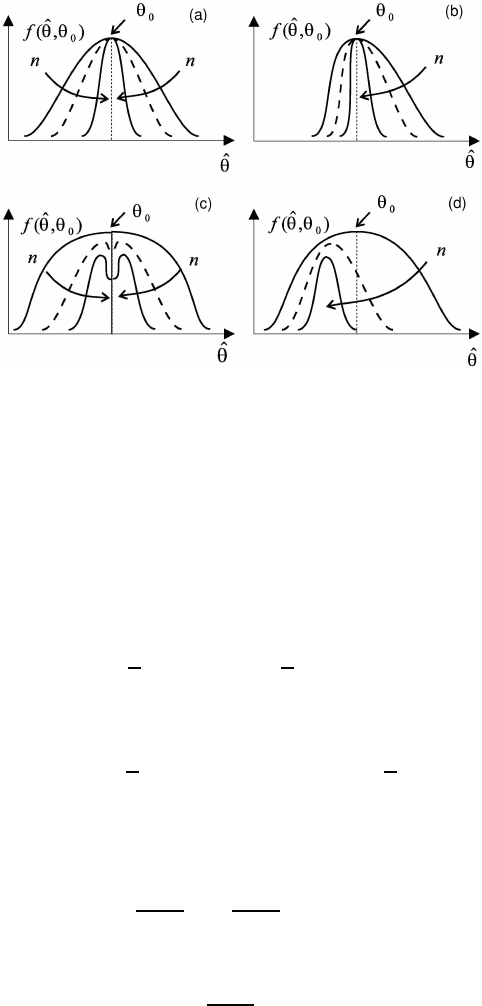
Fig. 2.3 Consistency and unbias. An estimate of a parameter

θ: unbias and consistent (a);

consistent, but bias (b); unbias, but inconsistent (c); inconsistent and unbias (d).

parameter θ, which can be bias, there is an asymptotically bias estimate, which sat-

isﬁes the condition M[

]

n→∞

−→ θ

. The mathematical expectation of such estimates

is tend to a right quantity of the parameter.

Example 2.6. Let for a repeated sample (x

, x

, . . . , x

) of normal observations

∈ N(m

, σ

) to ﬁnd an estimate for σ

Using the relation for a sample variance

i=1

− ¯x)

i=1

− ¯x

we obtain

M(s

) =

i=1

M[x

] − M [¯x

] =



1 −



So, the estimate of σ

is biased in the direction of smaller values. Obviously, that

the unbiased estimate of σ

can be written as

n − 1

i=1

− ¯x)

because

M[S

] =

n − 1

M[s

] = σ

The estimate s

is an asymptotically unbiased estimate of σ

, because M[s

]−σ

−σ

/n → 0 at n → ∞.

94 STATISTICAL METHODS OF GEOPHYSICAL DATA PROCESSING

2.2.3 Rao–Cramer inequality. Eﬃciency

An accuracy of the parameters estimation at a given number of observations and

an existence of the lower edge for the variance of the parameter was solved by S.

Rao and G. Cramer independently. They have proved the existence of the lower

edge for the variance of the estimate (Rao, 1972; Cramer, 1946).

Let us consider a case of a single parameter. Let the likelihood function

L(x

, x

, . . . , x

, θ) for a sample x

, x

, . . . , x

depends on the parameter θ, and

θ is an unbias estimate

θ =

θ(x

, x

, . . . , x

) of θ. The likelihood function satisﬁes

the normality condition

. . .

L(x

, x

, . . . , x

, θ)dx

, . . . , dx

= 1. (2.1)

Assuming permissible parameter diﬀerentiation of integrand, we obtain

. . .

∂L

∂θ

, . . . , dx

= 0. (2.2)

As the estimate

θ (M

θ = θ) is unbias, we have

. . .

θLdx

, . . . , dx

= θ, (2.3)

from which

. . .

∂L

∂θ

, . . . , dx

= 1. (2.4)

Taking into account the relations (2.2) and (2.4), we can write

. . .

[

θ − θ]

∂L(x

, . . . , x

, θ)

∂θ

, . . . , dx

= 1, (2.5)

. . .

[

θ − θ]



∂L

∂θ



Ldx

, . . . , dx

= 1. (2.6)

To rewrite the equality (2.6) as



(

θ − θ)



∂L

∂θ



= 1. (2.7)

To denote

θ − θ = V and (

)(∂L/∂θ) = W , and using an analog of the Cauchy–

Bunyakovckii inequality

M[V

] · M [W

] ≥ (M[V · W ])

we obtain

M[V

] · M [W

] ≥ 1 and M

(

θ − θ)

· M



∂L

∂θ



≥ 1. (2.8)

Elements of mathematical statistics 95

To implement a transformation of the expression M [(1/L)(∂L/∂θ)]. Let L 6= 0,

then

∂ ln L

∂θ

∂L

∂θ

∂

ln L

∂θ

= −



∂L

∂θ



∂

∂θ

. (2.9)

We multiply the expression (2.9) on L and, taking into account



∂

∂θ



. . .

∂

∂θ

, . . . , dx

= 0,

we obtain the equality for the mathematical expectations



∂L

∂θ



= −M



∂

ln L

∂θ



. (2.10)

Taking into account the equality (2.10), the inequality (2.8) can be rewritten as

θ)= M (

θ − θ)

≥

M[−∂

ln L/∂θ

]

. (2.11)

The inequality (2.11), which determine the lower edge for the variance of the pa-

rameter estimation, is called the Rao–Cramer inequality. A quantity



−

∂

ln L

∂θ



= M



∂ ln L

∂θ



= I

(F )

(θ) (2.12)

is the quantity of Fisher information, which has been introduced in Sec. 1.9.5. So,

the quantity of the Fisher information describes the lower edge for the variance of

the parameter:

θ] ≥ (I

(F )

(θ))

−1

. (2.13)

As mentioned above, this quantity does not depend on the way of the estimate

and it is the lower edge for the accuracy of an arbitrary estimate So, at given a

sample size the accuracy of the estimate has the bottom limit. In a case of the bias

estimate with bias b(θ) the Rao–Cramer inequality reads as

θ] ≥

1 + db/dθ

M [∂ ln L/∂θ]

, (2.14)

where b(θ) = M[

θ − θ].

In the case of repeated sample is valid

L(x

, . . . , x

, θ) = f

, θ)f

, θ) . . . f

, θ)

, θ) 6= 0, then

∂

ln L

∂θ

i=1

∂

ln f(x

, θ)

∂θ

96 STATISTICAL METHODS OF GEOPHYSICAL DATA PROCESSING

and



∂

ln L

∂θ



i=1



∂

ln f (x

, θ)

∂θ



= nM



∂

ln f (x

, θ)

∂θ



Since all quantities M



∂

ln f (x

, θ)/∂θ



are equal for all i, we obtain

θθ] ≥

nM [−∂

ln f (x, θ)/∂θ

]

(F )

(θ)

. (2.15)

In a case of a few parameters θθ = (θ

, . . . , θ

) the Rao–Cramer inequality reads

θθ] ≥ (I

(F )

(θθ))

−1

, (2.16)

where

θ] = kD

s,s

and I

(F )

(

θ) = kI

(F )

s,s

accordingly the covariance matrix for the estimates of parameters

= M

(

− θ

)(

− θ

)

and the Fisher information matrix

(F )

= M



−

∂

ln L(x,

θ)

∂θ



= M



∂ ln L(x,

θ)

∂θ

∂ ln L(xx,θθ)

∂θ



An estimate of the parameter

θ is called an eﬃcient estimate, if its variance

reaches own lower edge, i. e. the Rao–Cramer inequality transforms to the equality

θ] = (I

(F )

(θ))

−1

. (2.17)

As the eﬃciency measure a function

θ) = (I

(F )

(θ)D(

θ))

−1

, (2.18)

is used. This function has values from 0 up to 1, moreover for the eﬃcient estimate

θ) = 1. In the case of repeated observations the eﬃciency can be written as

θ) = nI

(F )

(θ)D[

θ]. (2.19)

The estimate is called as an asymptotic eﬃcient estimate, if e(

θ) → 1 at n → ∞.

Consider a case of the vector parameter θ. Let for the vector

VV = kV

s=1

an equality

s=1

= 1 is valid. Let project on it a random vec-

tor of estimates of parameters

θ = (

, . . . ,

). We get a random variable with

a variance V

θ)V

V and in accordance with the Rao–Cramer inequality we can

write

θ)V

V ≥

(F )

(

θ)]

−1

V . (2.20)

It means, that the correlation ellipsoid V

−1

(

θθ)

V = 1 of the random vector

θθ

envelops a ﬁxed ellipsoid V

(F )

(

θ)

V = 1. If the correlation ellipsoid of the system

of unbias estimates (

, . . . ,

) can be written as V

−1

(

θ)

V = 1 and coincides

with an ellipsoid V

(F )

(

θ)

V = 1, then (

, . . . ,

) is called the system of jointly

eﬃcient estimates. The system of jointly asymptotic eﬃcient estimates is deﬁned

as the consequence of the system of estimates (

, . . . ,

) for the parameters

(

, . . . ,

), which depend on a sample size n, asymptotically unbias and their

correlation ellipsoids

−1

(

θ)V = 1, at n → ∞ asymptotically tend to the

ellipsoid

(F )

(θ)VV = 1, which gives by the Fisher information matrix.

Elements of mathematical statistics 97

2.2.4 Suﬃciency

An estimate

θ(x

, . . . , x

) of the parameter θ is called a suﬃcient estimate, if the

likelihood function for a sample xx can be represented as

L(x

x, θ) = g(

θ, θ)h(

x), (2.21)

where h(x) does not depend on θ. In this case the conditional distribution of a vector

xx at ﬁxed

θ does not depend on θ, so the suﬃcient estimate

θ of the parameter θ

accumulates the complete information on θ, contained in the sample. The eﬀective

estimate necessarily is suﬃcient. The set of joint suﬃcient estimates (

, . . . ,

)

leads to the representation of the likelihood function as a product of functions

θ) = g(

θ, θ)h(x), (2.22)

where, as before, h(xx) does not depend on θ.

2.2.5 Asymptotic normality

Let us present n measurements (x

, . . . , x

) of random variables ξ with a density

function f

(x, θ), where θ is an unknown parameter. Let’s consider asymptotic

properties of the distribution of an estimate, which we shall consider as consistent.

Let’s take the advantage of the central limit theorem. From this theorem follows,

that

i=1

g(x

) (2.23)

at an asymptotic bound (n → ∞) has the normal distribution with the mathemati-

cal expectation M [g(

ξ)] and the variance D[g(ξξ)]/n, always supposing, that D[g(ξ)]

is a ﬁnite value. From the law of large numbers follows, that

i=1

g(x

)

n→∞

−→ M[g(ξ)] =

g(x)f(x, θ)dx. (2.24)

Supposing there is a such function g(x), that the right hand side of the equation

(2.24) is a known function q(θ):

M[g(ξ)] =

g(x)f(x, θ)dx = q(θ). (2.25)

If the equality (2.25) is valid for the true value θ

, there is an inverse function q

−1

for q, determined by the expression

−1

[q(θ

)] ≡ θ

. (2.26)

Using the equality (2.24), we obtain

= q

−1

{M[g(ξ)]}. (2.27)

98 STATISTICAL METHODS OF GEOPHYSICAL DATA PROCESSING

For a ﬁnding of an estimate

θ we shall take the advantage of the expression

θ = q

−1

(

i=1

g(x

)

. (2.28)

The expression (2.28) it is possible to take Taylor about a point M [g(ξ)]:

θ = q

−1

(

i=1

g(x

)

= q

−1

{M[g(ξ)]} +

∂q

−1

∂g

{M[g(ξ)]}

(

i=1

g(x

) − M [g(ξ)]

)

+ O(1/n).

At such order of the accuracy the estimate

θ asymptotically distributed under the

normal law N(θ

, D(

θ)) with an asymptotic variance

θ] = M

θ − θ

)



∂q

−1

∂g



D[g],

where D[g] is a variance g(ξ).

In the case of a vector of parameters

θ = (θ

, . . . , θ

), the functions g and q

−1

become the vector functions g and q

−1

accordingly. In this case matrix of the second

moments of an asymptotic distribution

θθ reads as

θ] = M

(

θ −

)(

θ −θθ

)



∂q

−1

∂gg





∂

−1

∂g



where D[g] is a matrix of second moments gg, ∂q

−1

/∂g is a matrix with the elements

∂

−1

/∂g

and q

−1

(

g) = θ

2.2.6 Robustness

Robust estimation is a such kind of estimation, which does not depend on a type of

the distribution or insensitive to the deviation from the guessed distribution. As a

rule, at processing the experimental geophysical data the normality of an errors of

measurements is supposed. The great outliers lead to the deviation from the normal

distribution. The robust procedure allows to exclude the inﬂuence of great errors

(examples of robust procedures see in the Sec. 6.14).

In addition to the mentioned above desirable properties of estimates of sought

for parameters (consistence, unbiasedness, eﬃciency, normality, robustness), at the

practical realization of a method of an estimation the essential factors are compu-

tational complexity of a method at the processing of the bulk of the geophysical

information and the computation time.

Chapter 3

Models of measurement data

At the design of the geophysical experiment and the interpretation of its data the

concept of a model is a basic concept. The success of the prognosis of a geological

structure of an explored parcel of the Earth crust substantially depends on the

chosen model. In the geophysical literature there are various aspects of the use

of the concept of the model. At the ﬁrst, the notion of the model is connected

with the concrete a priori assumptions concerning a structure of one or another

geophysical object. For example, the layered model of the medium is a basis of

many methods of the processing of the seismic data: build-up of a pseudo-acoustic

impedance section with the purpose of the prediction of a geological section; the

migration of a seismic time section in the depth section etc. In more complicated

geological conditions is possible to use models of an anisotropic layered medium, in

which the velocity of the propagation of the seismic waves depends on a direction of

the propagation. In a case of a magnetometry and a gravimetry an example of such

models can be an object with a priori assigned shape, which creates an anomalous

magnetic or a gravitational ﬁeld. Secondly, the concept of the model includes a

priori assumptions about the connection between the observed experimental ﬁeld

and parameters, interesting for the investigator, and conditions of a parcels of the

Earth’s crust, thus the random character of experimental data should be taken into

account. The explored geological object is a complicated multiparameter system,

and for its study it is necessary to take all available geological and geophysical

information. At the analysis of real objects the principle of a “black box”, which

guess a complete absence of a priori information is completely unacceptable.

3.1 Additive Model

Let’s suppose that the observation of a geophysical ﬁeld u will be carried out in a

Cartesian frame (x, y, z) in discrete points of the space (x

, y

, z

) in instants t

where k = 1, . . . , K, l = 1, . . . , L, m = 1, . . . , M, i = 1, . . . , n. If a step at measuring

is uniform, then x

= k∆x, y

= l∆y, z

= m∆z, t

= i∆t, where ∆x, ∆y, ∆z, and

∆t are the quantization steps on the space and time accordingly. The important

100 STATISTICAL METHODS OF GEOPHYSICAL DATA PROCESSING

special case of a system of observations are the measuring along a linear proﬁle,

when, combining an axis 0x with a direction of the proﬁle, we shall obtain for a

seismic ﬁeld u(x

, t

) and for a magnetic or a gravitational ﬁeld we shall obtain

u(x

On the basis of the available a priori information an investigator creates the

model of the medium, which allows with the use of the physical laws to establish a

functional connection between desired parameters of the medium

θ = (θ

, . . . , θ

where S is a number of desired parameters, and a model ﬁeld on a observation

plane f (θ

θ, x

, y

, z

, t

). Thus, a random component of the model ε(x

, y

, z

, t

) is

functionally connected with the the model ﬁeld and the observed ﬁeld:

u(x

, y

, z

, t

) = Φ(f(x

, y

, z

, t

θ), ε(x

, y

, z

, t

)). (3.1)

The additive model has a greatest prevalence in a practice of the processing of

the geophysical data. In a case of this model a functional connection Φ corresponds

to a simple superposition of a model ﬁeld f and a random component of the model

ε:

u(x

, y

, z

, t

) = f(x

, y

, z

, t

,θ

θ) + ε(x

, y

, z

, t

). (3.2)

Such representation points to the independence of sources of a model ﬁeld and

noise. Using the formula (3.2) for a seismic trace, we guess, that f includes the wave

ﬁeld, computed according to the accepted model of the medium, and ε is the con-

tribution of a microseism, a noise of the received chain, geological inhomogeneities

unaccounted in a model ﬁeld. For problems of the magnetometric prospecting and

gravimetric prospecting the possible example of a such model can be written as

a superposition of a model ﬁeld f of the object of the known sample shape (for

example, layer, bench etc.) and a random ﬁeld ε, which is caused by errors of ob-

servations, the inﬂuence of non interpretive sources of a ﬁeld, and also errors, which

is connected with a replacement of the real magnetic object by its physical analog.

The model (3.2) can be obtained from a general model (3.1) by a linearization

at a small enough ε. The parameters θ, included in model, depending on a physical

statement of a problem can be either unknowns values, or random values, thus the

various algorithms of estimations of parameters are used. At the formalization of a

model, together with the physical basis, it is necessary to take into account a com-

puting complexity and a practical realizability of the chosen approach. Further the

models as with known (but not random), and with random parameters will be used.

Let’s mark, that the representation about a random character of an experimental

material underlies the statistical theory of the interpretation and determines the

concrete algorithm and the eﬃciency of a processing algorithm. It is necessary to

underline, that the information substance of the interpretation becomes up to the

extremely clear only within the framework of the statistical theory, in which the

gained information is determined by a diﬀerence of entropies of a priori probability

distributions (before interpretation) and a posteriori probability distributions (after

interpretation) about a state of the object. So a random character of inferences thus

admits which is a direct consequence of a random character of measurements.

Models of measurement data 101

3.2 Models of the Quantitative Interpretation

The model (3.2) belongs to the set of models of the quantitative interpretation.

The function f(x

, y

, z

, t

, θ) is supposed to be known and is determined by the

physical problem statement. The problem consists in a ﬁnding of an estimate of

parameters

θ on a given experimental material u(x

, y

, z

, t

), that corresponds to

procedure of a point estimation of the parameters in the terms of a mathematical

statistics.

As an example of a such model we shall consider a model of a seismic trace:

u(t

) =

µ=1

ϕ(t

− τ

) + ε(t

), (3.3)

with the vector of sought for parameters θ

θ = kA

, τ

µ=1

. At that time-continuous

analog of the model (3.3) can be written as

u(t) =

µ=1

ϕ(t − τ

) + ε(t). (3.4)

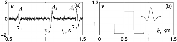
An example of the seismic trace is represented at Fig. 3.1.

Fig. 3.1 An example of the seismic trace: (a) it is seismic trace with the Gaussian noise

(N(0, 0.1)); (b) depth dependence of velocity of the wave propagation and the time dependence in

a seismic source. Observation point is located near the free surface.

In some problems of the data processing it is expedient to carry out the analysis

in the frequency domain. Using the Fourier transform, the model (3.4) is possible

to rewrite as

u(ω) =

µ=1

Φ(ω) exp{−iωτ

} + E(ω), (3.5)

where

u(ω) =

∞

−∞

u(t) exp{−iωt}dt,

Φ(ω) =

∞

−∞

ϕ(t) exp{−iωt}dt,

E(ω) =

∞

−∞

ε(t) exp{−iωt}dt.

102 STATISTICAL METHODS OF GEOPHYSICAL DATA PROCESSING

In the case of the model (3.3) we use the discrete Fourier transform or Z-transform

(Z = e

−iω∆t

u(z) =

µ=1

Φ(z)z

/∆t

+ E(z),

u(z) =

i=0

, Φ(z) =

i=1

, E(z) =

i=0

. (3.6)

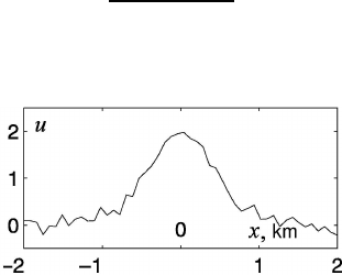
Let’s consider an example from a magnetometry. Let a vertical component of a

magnetic ﬁeld u(x

) is registered along a linear lateral proﬁle in points x

is caused

by a vertical magnetic dipole, then a linear model of the experimental ﬁeld can be

written as

u(x

) =

M(2h

− x

)

+ h

)

5/2

+ ε(x

), (3.7)

where M is a magnetic moment of the dipole, h is an occurrence depth (Fig. 3.2).

Fig. 3.2 Magnetic ﬁeld with the Gaussian (N (0, σ

)) noise (3.7) along the linear lateral proﬁle

(h = 1, M = 1, σ = 0.1).

3.3 Regression Model

At the processing of the geophysical information the interpreter frequently confronts

with a problem of the smoothing of the initial or the intermediate data by functions

of a given degree of a smoothness. So, for example, at the calculation of the normal-

moveout spectrum of velocities with the purpose of the deﬁnition of the velocity

CDP

the hodograph of a wave is approximated by a parabola of the second order

the similar approximation of a hodograph is used also at a static correction. For

extraction of the local magnetic or gravity anomalies it is necessary to remove the

inﬂuence of a regional background, which can be circumscribed by a smooth surface.

The similar problem arises at the analysis of structural maps obtained on the data

of a seismic exploration, where it is necessary to extract an anticline with a small

amplitude on a background of a regional raising. These and many other problems

are solved by the regression analysis.