Труды Всемирного конгресса Международного общества солнечной энергии - 2007. Том 2
Подождите немного. Документ загружается.


COMPARISON OF SEVEN SOLAR AIR-CONDITIONING SYSTEMS
INSTALLED IN DIFFERENT COUNTRIES
He Zinian
Beijing Solar Energy Research Institute,
10 Dayangfang, Beiyuan Road, Chaoyang District
Beijing 100012, China
solarthe@public.bta.net.cn
Li Wei, Wang Ling
Beijing Sunda Solar Energy Technology Co., Ltd,
3 Huayuan Road, Haidian District
Beijing 100083, China
liwei@beijingsunpu.com.cn
ABSTRACT
Seven solar air-conditioning systems using heat-pipe
evacuated tube collectors or direct-flow evacuated tube
collectors have been installed in different countries since
1998. The collectors were developed by Beijing Solar
Energy Research Institute and manufactured by Beijing
Sunda Solar Energy Technology Co., Ltd. These seven
solar air-conditioning systems have a collector range from
82m
2
to 680m
2
and a cooling capacity range from 36kW to
560kW. Furthermore, design features, measuring
performances and operation result for five solar
air-conditioning systems are described in more detail.
1. INTRODUCTION
Electric power required for providing air-conditioning takes
a very large portion of total electric power consumption in
the world. For this reason, various solar air-conditioning
systems have been investigated and installed. Solar
air-conditioning has an obvious advantage that the most
cooling demand is just matched with the strongest solar
irradiation in summer reason, which attracts more and more
attention from many countries worldwide.
Heat-pipe evacuated tube collectors (ETC) and direct-flow
ETC developed by Beijing Solar Energy Research Institute
and manufactured by Beijing Sunda Solar Energy
Technology Co., Ltd, have been used for solar
air-conditioning since 1998. This paper will briefly
introduce configurations and characteristics of these two
kinds of ETC.
Seven solar air-conditioning systems with different
installation scales were successively installed in different
countries. This paper will summarize and compare their
installation scales, technical specifications and chiller
models. Among them, six systems adopt absorption chiller
and one system adopts adsorption chiller. Some of them
have multifunction with solar space cooling in summer,
solar space heating in winter and solar domestic water
heating in other seasons, so as to obviously enhance
economical benefit of the solar air-conditioning system.
In addition, this paper will describe in more detail the
hydraulic scheme, design features, measuring performances
and operation results of five solar air-conditioning systems
respectively installed in Stuttgart of Germany, Rushan of
China, Freiburg of Germany, Beijing of China and Los
Angeles of the United States.
2. EVACUATED TUBE COLLECTORS
According to sorts of material for absorber, ETC could be
classified into one with a metal absorber and the other with
a glass absorber. Beijing Sunda only produces the ETC
with metal absorbers because they possess some common
advantages, such as high-pressure bearing and thermal
shock endurance, both of which are very necessary for most
solar thermal systems. Two main products -- heat-pipe ETC
3 SOLAR COLLECTOR TECHNOLOGIES AND SYSTEMS
843
and direct-flow ETC are briefly described below. [1]
2.1 Heat-pipe ETC(SEIDO1,5,10)
The heat-pipe ETC involves several heat-pipe evacuated
tubes. Each heat-pipe evacuated tube is mainly composed
of heat pipe, absorber plate, glass envelope tube, metal
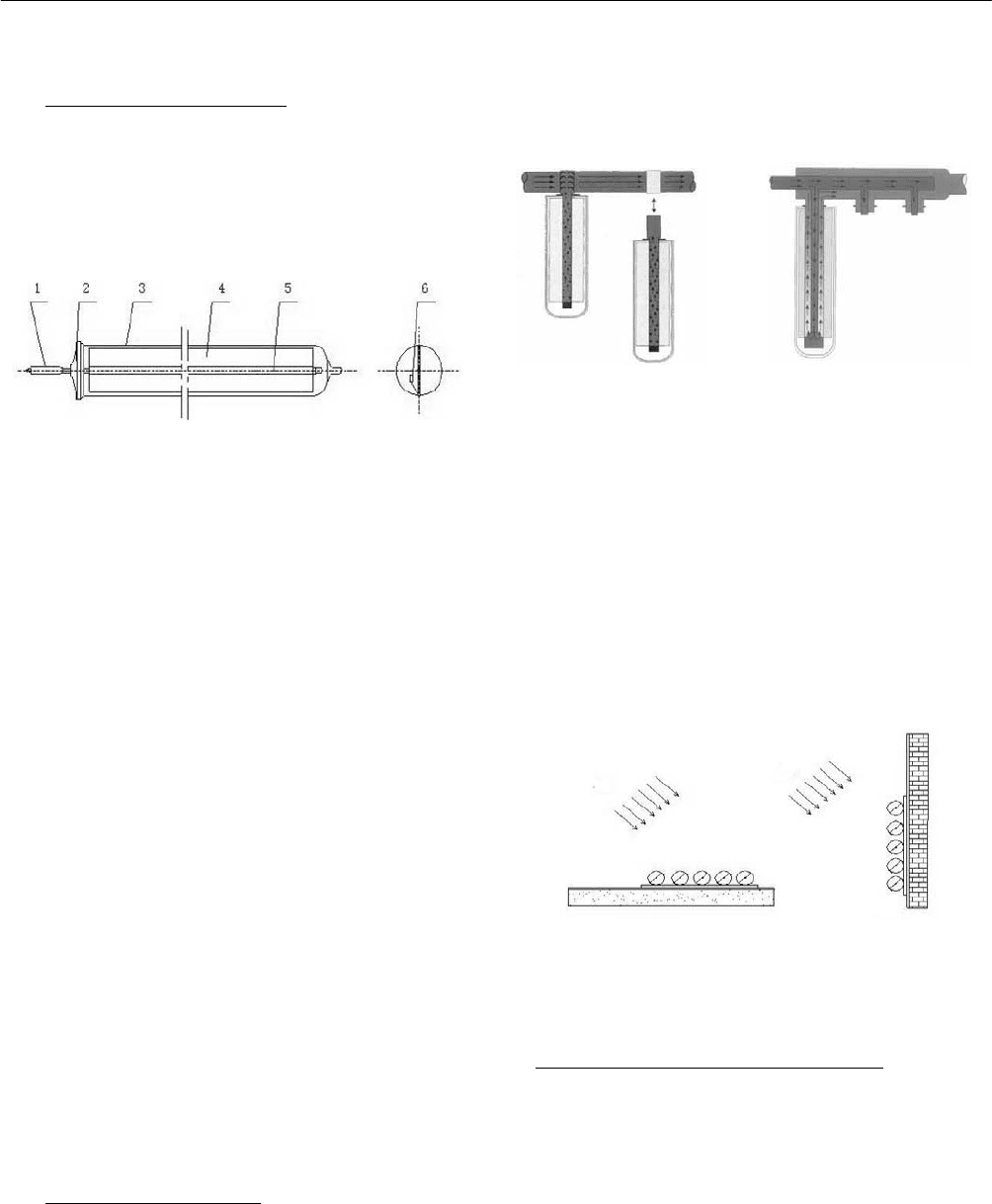
sealing cover, getter and others, as shown in Fig. 1.
1. Heat-pipe condenser section 2. Metal sealing cover
3. Glass envelope tube 4. Absorber plane
5. Heat-pipe evaporator section 6. Getter
Fig. 1: Configuration of heat-pipe evacuated tube.
The heat-pipe ETC consists of evacuated tubes, manifold,
insulation box and other accessories, as shown in Fig. 2.
Evacuated tubes are separated from the heating circuit by
means of “dry connection”, so that individual tubes can be
easily replaced at any time whenever necessary without
interrupting operation of the solar system and without water
leakage problem as well.
As heat pipe technology is applied to evacuated tube and
heat transfer fluid of the collector does not pass through
evacuated tubes, therefore the heat-pipe ETC has many
advantages, such as anti-freeze due to effective measures
adopted for the heat-pipe, fast start-up due to small heat
capacity of working fluid in the heat-pipe, low heat losses
due to “thermal diode effect” of the heat-pipe,
high-pressure bearing and thermal shock endurance due to
“dry connection” between evacuated tubes and the
manifold, etc.
To meet different requirements, several types of heat-pipe
ETC have been developed as SEIDO1, SEIDO5 and
SEIDO 10.
2.2 Direct-flow ETC(SEIDO2)
The direct-flow evacuated tube SEIDO2 is very similar to
the heat-pipe evacuated tube SEIDO1 in appearance,
dimensions and configuration except the concentric pipes
instead of the heat-pipe. SEIDO2 ETC consists of
evacuated tubes, manifold, insulation box and other
accessories, as shown in Fig. 3.
Fig. 2: Structure of heat- Fig. 3: Structure of direct-
pipe ETC.
flow ETC.
The direct-flow ETC has many advantages, such as higher
thermal efficiency due to direct heat removal, high-pressure
bearing and thermal shock endurance due to metal absorber
plate, etc. In addition, the direct-flow ETC can be either
horizontally installed on a flat roof or integrated onto a
facade of the building, as shown in Fig. 4. In these cases,
SEIDO2 evacuated tubes together with absorber plates
should be turned towards the sun with their optimal tilted
angle.
(a) On flat roof (b) On facade
Fig. 4: Flexible installation of direct-flow ETC.
3. SOLAR AIR-CONDITIONING SYSTEMS
Since 1998, seven solar air-conditioning systems have been
installed in Germany, Japan, China, USA and India
respectively. The installation scales, technical specifications
and chiller models of seven solar air-conditioning systems
are shown in Table 1.
Proceedings of ISES Solar World Congress 2007: Solar Energy and Human Settlement
844
These solar air-conditioning systems have a collector range
from 82m
2
to 680m
2
and a cooling capacity range from
36kW to 560kW. Among them, six systems adopt
absorption chiller and one system adopts adsorption chiller.
The heat-pipe ETC used for these systems include SEIDO1,
SEIDO5 and SEIDO10.
4. MAIN FEATURES OF SOLAR A/C SYSTEMS
To understand these systems in more detail, the design
features, measuring performances and operation results of
following five solar air-conditioning systems are described.
4.1 Stuttgard System (Germany)
The solar air-conditioning system was installed in the
Meissner & Wurst Company in Stuttgart, Germany. The
system adopts SEIDO1 heat-pipe ETC, which are installed
on a flat roof with a hall of triangular cross section, as
shown in Fig. 5. A lithium-bromide absorption chiller is
used for the cooling system.
The solar collector array supplies hot water at about 95 ć
to an inlet of the chiller. The chiller produces chilled-water
at about 6 , and the water return to the chiller at aboć ut
12 .ć
Fig. 5: Solar A/C system in Stuttgart, Germany.
4.2 Rushan System (China)
Rushan is located at the southeast end of Shandong
Peninsula. In this area, the maximum air temperature in
summer is 33.1ć and the minimum air temperature in
winter is –7.8ć. Under the local climate, both space
cooling in summer and space heating in winter are required
for comfort.
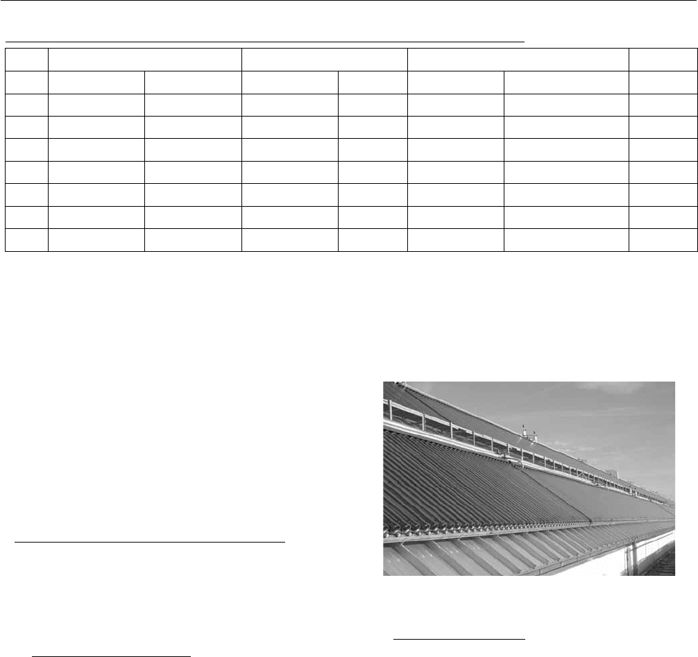
The solar air-conditioning system was installed in the Solar
Energy Hall of the Chinese Renewable Energy Popular
Science Park.
The Hall is a two-story building with a
construction area over 1000m
2
and has been architecturally
designed to meet requirements of solar collector array
TABLE 1: MAIN SPECIFICATION OF SEVEN SOLAR AIR-CONDITIONING SYSTEMS
NO LOCATION SOLAR COLLECTOR CHILLER YEAR
City Country Type Area (m
2
) Type Cooling cap. (kW)
1 Stuttgart Germany SEIDO 1 320 Absorption 560 1998
2 Hirohima Japan SEIDO 1 228 Absorption 140 1998
3 Rushan China SEIDO 5 432 Absorption 100 1999
4 Freiburg Germany SEIDO 2 170 Adsorption 70 2001
5 Beijing China SEIDO 1 680 Absorption 360 2004
6 Los Angeles USA SEIDO 1 82 Absorption 36 2004
7 Kalol India SEIDO 10 162 Absorption 90 2006
Note:
SEIDO 1 Heat-pipe ETC with flat absorber plate,¶100mmh2000mm
SEIDO 5 Heat-pipe ETC with semi-cylindrical absorber plate,¶100mmh2000mm
SEIDO 10 Heat-pipe ETC with flat absorber plate,¶70mmh1750mm
SEIDO 2 Direct-flow ETC with flat absorber plate,¶100mmh2000mm
3 SOLAR COLLECTOR TECHNOLOGIES AND SYSTEMS
845
placement, as shown in Fig. 6.
[2]
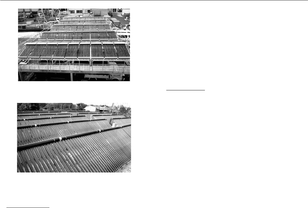
Fig. 6: Full view of the solar A/C system in Rushan, China.
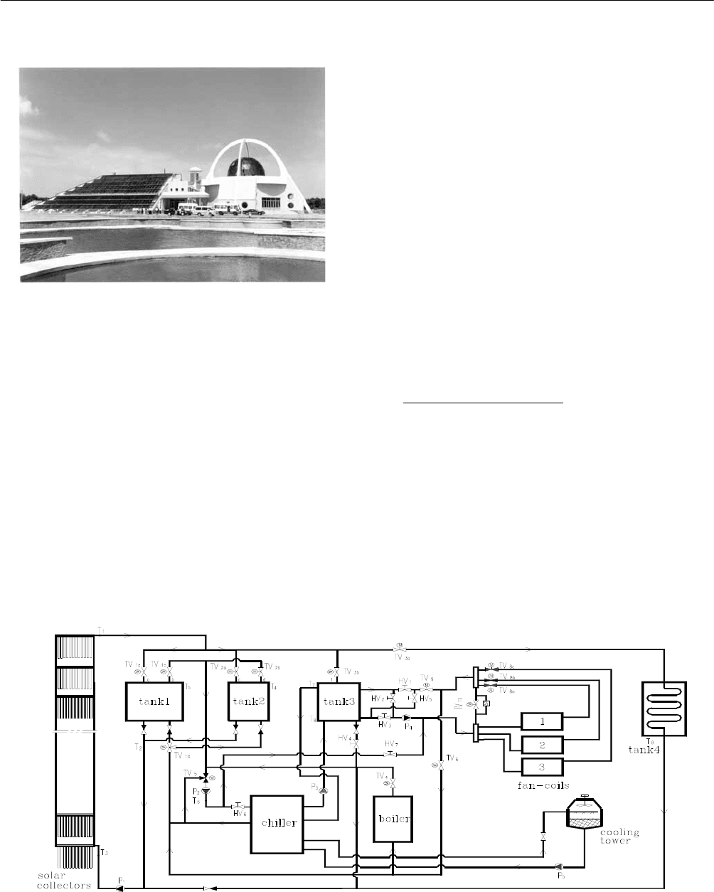
A layout of the system is shown in Fig. 7. The solar
air-conditioning system consists of SEIDO5 heat-pipe ETC
array, lithium-bromide absorption chiller, cooling tower,
water storage tanks, circulating pumps, fan-coil units,
auxiliary oil-burned boiler and control device.
To obtain more solar irradiation over a day, evacuated tubes
with a semi-cylindrical absorber plate were selected.
Theoretical calculation and measuring data show that the
semi-cylindrical absorber plate increases 10-14% more
energy output than the flat absorber plate.[3]
The absorption chiller has a maximum cooling capacity of
176 kW (50 USRT). The solar collector array supplies hot
water at about 88 to an inlet of the chiller and the water ć
leaves the chiller at about 83 . ć The COP (Coefficient of
Performance) of the chiller is approximately 0.70. The
chiller produces chilled-water at about 8ć and the water
return to the chiller at about 13 . The cooling water ć
temperature through the chiller is successively 31 and ć
37 .ć
There are totally four storage tanks in the system. The tank
1 and tank 2 are used to store the hot water produced by the
solar collector array. The smaller tank 2 aims to reach a
specified temperature value for the chiller in the early
morning. The tank 3 is used to store the chilled-water to
reduce heat losses of the storage tank, because temperature
difference between ambient temperature and chilled-water
temperature is much smaller than that between hot-water
temperature and ambient temperature.
4.3 Freiburg System (Germany)
The solar air-conditioning system was installed in one of
the laboratories in University of Freiburg.[4] The system
adopts SEIDO2 direct-flow ETC, which are horizontally
installed on a flat roof, as shown in Fig. 8. All evacuated
tubes with absorber plates are turned towards the sun with a
tilted angle 45°. An adsorption chiller with silica gel is used
for the cooling system.
Fig. 7: Layout of the solar A/C system in Rushan, China.
Proceedings of ISES Solar World Congress 2007: Solar Energy and Human Settlement
846
Fig. 8: Solar A/C system in Freiburg, Germany.
Through measurement, COP of the adsorption chiller was
in the range of slightly above 0.50, and COP had a
maximum when operating temperature of the solar
collector array was about 71ć. In total, the supplied solar
heat accounted about 78% of the required driving heat.
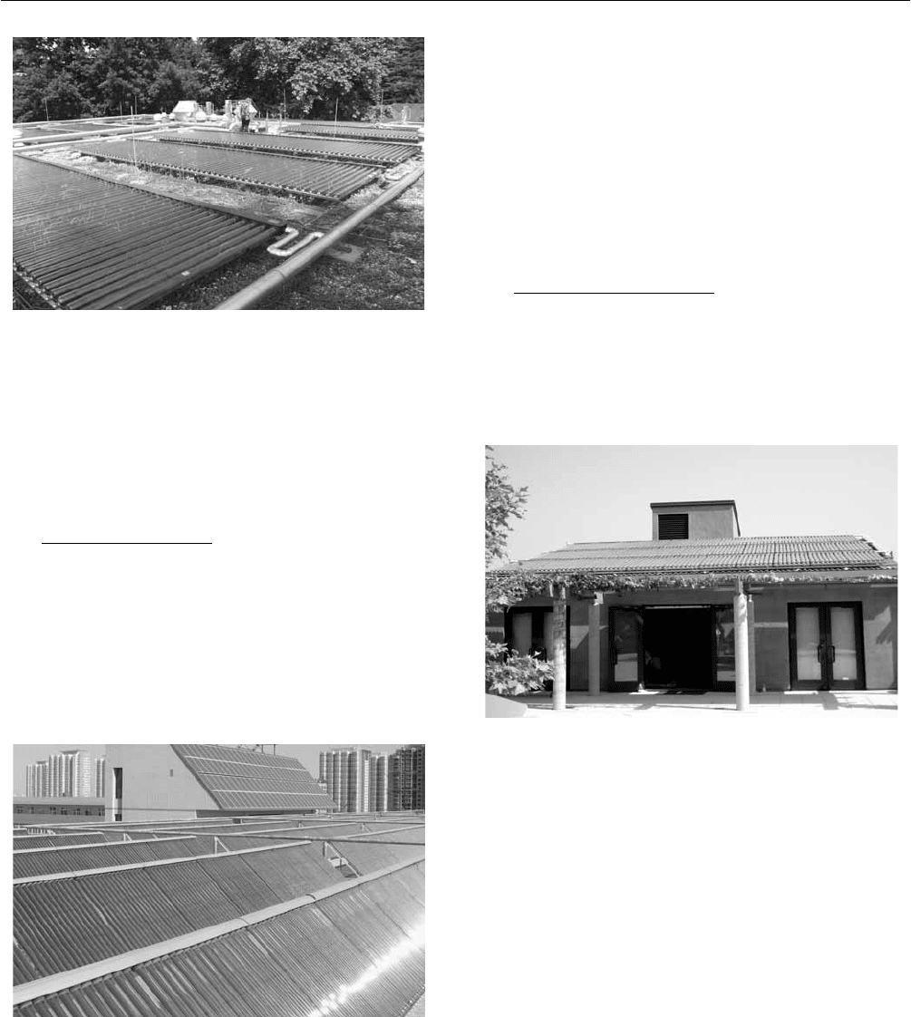
4.4 Beijing System (China)
Fig. 9 shows the solar air-conditioning system installed in an
office building of Beijing Solar Energy Research Institute.
SEIDO1 heat-pipe ETC is used for the system. The layout
and main features of the system are similar to that for the
Rushan system. A lithium-bromide absorption chiller has a
maximum cooling capacity of 360 kW (100 USRT).
Fig. 9: Solar A/C system in Beijing, China.
The system has been selected as one of the national
demonstration projects in China. From one-year monitoring
test results, in the air-conditioning period, the daily useful
energy gain reached 5760 MJ-8350 MJ, the daily average
collector efficiency reached 41%-50% and the overall solar
fraction was 82%; in the space heating period, the daily
useful energy gain reached 4750 MJ-8240 MJ, the daily
average collector efficiency reached 39%-52% and the
overall solar fraction was near 79%, so that the system
could meet most of air-conditioning requirements in
summer and space heating requirements in winter.
4.5 Los Angeles System (USA)
The solar air-conditioning system was installed at Audubon
Urban Nature Center in Los Angeles, USA. The system
adopts SEIDO 1 heat-pipe ETC, which are installed on a
slope roof, as shown in Fig. 10.
Fig. 10: Solar A/C system in Los Angeles, USA.
The absorption chiller has a maximum cooling capacity of
36 kW (10 USRT). The solar collector array supplies hot
water at about 88 to the chiller. COP of the chiller is ć
approximately 0.70. The chiller produces chilled-water at
about 9 . The cooling water temperature through the ć
chiller is about 30ć. A small amount of electric power to
run the pumps and fans is supplied by solar photovoltaic
panels.
Fig. 11 and Fig. 12 show solar air-conditioning systems
respectively installed in Hirohima, Japan and in Kalol,
India. Unfortunately, there are no more detailed data
available.
3 SOLAR COLLECTOR TECHNOLOGIES AND SYSTEMS
847
Fig. 11: Solar A/C system in Hirohima, Japan.
Fig. 12: Solar A/C system in Kalol, India.
5. CONCLUSIONS
The practice has proved that both heat-pipe ETC and
direct-flow ETC are very suitable for solar air-conditioning
systems.
The heat-pipe ETC could be operated at 88ć to 95ć,
which are favourable to increase COP of the chiller.
Meanwhile, the heat-pipe ETC still could have daily
average efficiency over 40%.
6. REFERENCES
(1) He Zinian, Advanced evacuated tube solar collectors-
Products and applications [J], Asia-Pacific Tech
Monitor, 2003, Nov-Dec, 42-47
(2) He Zinian, Demonstration of a Solar Absorption
Air-conditioning System Powered by Heat-pipe
Evacuated Tubular Collectors, Proceeding of EuroSun
2000 Congress, Copenhagen, Denmark, 2000.
(3) He Zinian, Ge Hongchuan, Jiang Fulin, Li Wei. A
Comparison of Optical Performance between
Evacuated Collector Tubes with Flat and
Semi-cylindrical Absorbers [J], Solar Energy, 1997, 60,
109-117
(4) Hans-Martin Henning, Hendrik Glaser, Solar Assisted
Adsorption system for a Laboratory of the University
Freiburg, 2003

ON THE VALIDATY OF A DESIGN METHOD TO ESTIMATE THE SOLAR
FRACTION FOR AN EJECTOR COOLING SYSTEM
Sergio Colle
LEPTEN / LABSOLAR – Department of Mechanical
Engineering - Federal University of Santa Catarina
88040-900
Florianópolis, SC, Brazil
colle@emc.ufsc.br
Guilherme dos Santos Pereira
LEPTEN / LABSOLAR – Department of Mechanical
Engineering - Federal University of Santa Catarina
88040-900
Florianópolis, SC, Brazil
Humberto Ricardo Vidal Gutiérrez
Department of Mechanical Engineering - University of Magallanes
P.O.Box 113-D
Punta Arenas, Chile
humberto.vidal@umag.cl
ABSTRACT
The present paper is concerned with the simulation of an
ejector cooling system in order to investigate the validity of
a design method to estimate the solar fraction. The cooling
capacity of the ejector cycle is assumed to be constant
during day periods. The ejector is assumed to steadily
operate at its optimum efficiency point. The solar fraction
derived from hourly simulation of the system is compared
with estimates obtained by the
chartf −− φ method based
on the utilizability concept. An equivalent minimum
temperature for the utilizability of the solar system is found,
which is proved to be different but close to the vapor
generator temperature of the ejector cycle.
1. INTRODUCTION
Global effort has insofar been devoted to develop
renewable energy systems in favor of CO
2
emission
reduction. Solar energy has been considered worldwide as
an effective alternative, to reduce fossil fuel and electric
energy consumption in domestic water heating application.
Flat plate collectors and evacuated collectors are proven to
be cost effective for many applications in domestic and
industrial process heat, for temperatures less than 100
o
C.
On the other hand, solar driven cooling cycles are hardly
competitive with mechanical compression cycles. There are
few real situations where solar driven absorption cooling
systems can be competitive with mechanical compression.
Capital cost of solar collectors and barriers arising from
architecture constraints contribute to reduce the economical
advantages in favor of absorption cooling cycles.
Furthermore, mechanical compressors have become
cheaper and more efficient in the past ten years. The
situation is not better for ejector cooling cycles. The
coefficient of performance (COP) of a single stage
absorption chiller of lithium bromide – water can easily
reach 0.66 while the COP of an ejector cycle, under the
same operation temperatures hardly reaches 0.6. The lower
the COP the greater the optimum collector area needed to
meet the load requirements. Therefore the potential
advantages arising from the lower cost of an ejector cooling
system is impaired by the requirement of additional
collector area.
The ejector system has usually to be simulated in the hourly
basis, with the help of Typical Meteorological Year (TMY)
3 SOLAR COLLECTOR TECHNOLOGIES AND SYSTEMS
849
database. TMY database are usually available in the
meteorological services of any developed country. However,
qualified TMY database are hardly available in developing
and undeveloped countries. On the other hand, monthly
averages of global and beam solar radiation incident on
horizontal surface became accessible by most of the
countries, thanks to the well succeed techniques to estimate
incoming solar radiation derived from satellites, as reported
in [1]. The incoming radiation can presently be estimated
with uncertainty around 5% against ground truth data [2].
For the above reasons, the design
chartf −− φ method, as
proposed in [3], based on monthly average solar radiation,
is still useful to design and optimize solar cooling systems,
as well as to analyze the economical feasibility of theses
systems for given economical scenarios. These methods
have been successfully used in designing systems to
provide process heat, as well as for cooling applications, as
reported in [4]. In [4] is presented an analysis of an
optimized ejector cooling system, reporting the results of
simulation based on hourly data, with comparison with the
predictions given from the
chartf −− φ method.
The present paper reports simulation results to show that
the
chartf −− φ method of can be validated in terms of
the monthly and annual solar fraction. The validation was
carried out for the city of Florianopolis – Brazil (latitude
27,6 South) for which a TMY database is available. The
database was built from a fourteen years long solar
radiation data series collected in a BSRN surface station [5].
The
chartf −− φ method is applicable to cases for
which the heat is supplied to the load only when the heating
fluid temperature is above some minimum temperature
min
T . It means that the method is expected not to be valid in
the circumstance the process heat depends on the
temperature of the loading system. In the case of an ejector
cooling cycle, the process heat depends not only of the
condenser temperature, but also on the vapor generator
temperature. As is shown in this paper, the
chartf −− φ
method can be validated for ejector cooling systems, once a
minimum temperature around the temperature of the vapor
generator is properly chosen.
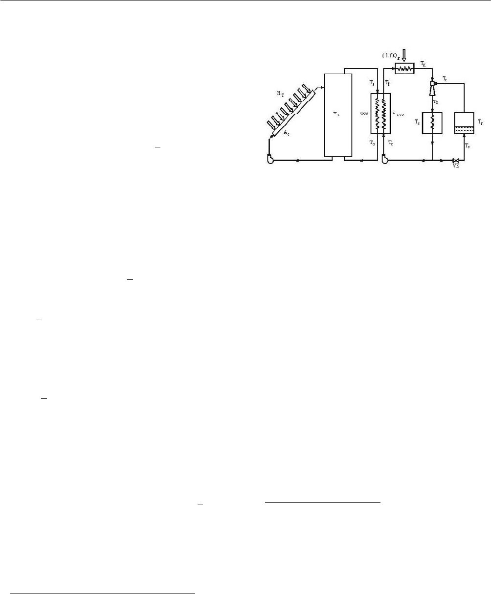
2. THE EJECTOR SOLAR COOLING SYSTEM
The ejector solar cooling system is conceived as a solar
heating system which supplies heat to an ejector cooling
cycle as shown in Fig. 1.
Storage
tank
Solar
collector
Auxiliary
burner
Condenser
Evaporator
Pump
Pump
Ejector
Expansion
valve
Va p o r
generator
Fig 1: Solar assisted ejector cooling system.
The working fluid evaporates in the vapor generator at the
saturation temperature
g
T to provide the primary stream
to the ejector nozzle. The mixture of the primary stream
with the secondary stream coming from the evaporator at
r
T , condenses in the condenser at temperature
c
T . The
condensed liquid stream leaves the condenser and splits
into two streams, one that flows back to the evaporator
though the expansion value, and the other that flows back
to the vapor generator. The ratio of the primary to the
secondary nozzle cross section areas of the ejector are
designed in order to achieve the maximum flow ratio in the
evaporator, for a given flow ratio of the primary stream.
Algorithms for simulation and optimization of the ejector
nozzle operation can be found in [6,7,8]. It is assumed here
that auxiliary heat is provided to the ejector system through
a burner, whenever the heat from the solar collector is not
enough in order to meet the load requirements, so that the
steady state flow rate of the refrigerant working fluid is
assured.
3. GOVERNING EQUATIONS
The full mixing model is assumed here in order to simplify
the energy balance of the solar system considered. In other
words, it is assumed there is no temperature gradient in the
storage tank, as well as no pressure and temperature drop in
the system pipes.
The energy balance in the solar system conjugated to the
vapor generator of the ejector cycle leads to the following
ordinary differential equation

Proceedings of ISES Solar World Congress 2007: Solar Energy and Human Settlement
850
() () ( )
[]
()( )
ssaiss
aesLRTnRc
s
s
QTTUA
TTUFGKFA
dt
dT
cm
α
τα
τα
−−−
−−=
(1)
where
s
T is the temperature of the heating fluid in the
storage tank,
sp
)mc( is the thermal capacity of the heating
fluid in the storage tank,
nR
)(F τα and
LR
UF are
respectively the energy gain and loss coefficient of the
straight line correlation of the flat plate collector efficiency,
c
A is the useful collector area,
s
)UA( is the heat loss
coefficient of the storage tank
)K/kW( ,
ai
T and
ae
T
are the ambient temperatures for the storage tank and solar
collector, respectively,
)m/W(G
T
2
is the solar radiation
incident on the tilted collector,
τα
K is the incidence angle
modifier of the collector,
COP/QQ
rg
= is the heat
input of the cooling cycle
)kW( , where
r
Q is the cooling
capacity, and COP is the coefficient of performance of the
ejector, which is a function of
c
T ,
g
T , and
r
T . Here
s
α
is a flag set to vanish for
cs
TT ≤ and set equal to the unity
for
cs
TT > . The vapor generator is considered to be a
two-phase heat exchanger, so that two distinct cases should
be considered as follows.
The hourly solar fraction is defined by
gs
Q/Qf = . The
annual solar fraction
a
f is the average of the hourly solar
fraction
f based on the sum of the hours of the day
duration in the year.
Case I
: Single-phase heat supply )TT(
gf
< .
In this case the heat input to equation (1) is given by
()
(
)
cfrlejcssmins
TTcTTWQ −=−= ωε (2)
where
s
ε the single-phase heat exchanger effectivity
defined as
(
)
()
csmincfrlejs
TTW/TTc −−= ωε (3)
where
ej
ω is the mass rate of the refrigerant,
rl
c is the
specific heat of the subcooled refrigerant,
min{( ) , }Wccωω= , where
sp
)c(ω is the hourly
thermal capacity of the heating fluid. The effectivity
s
ε is
a function of
s
)UA( and /WW, where
s
)UA( is
the product of the global heat transfer coefficient and the
single-phase heat exchanger area
s
A , which must be equal
to the total heat exchanger area
TCS
A . The heating fluid
temperature
sl
T corresponding to the situation for which
the refrigerant temperature reaches
g
T , by equation (2) is
given by
(
)
smincgrlejcsl
W/TTcTT εω −+= (4)
While
f
T remains lower than
g
T (and therefore
s
T remains lower than
sl
T ) the heat input is given by
equation (2) .
Equation (1) with the input
s
Q given by equation (2), can
numerically be solved up to the time for which
s
T reaches
sl
T .
Case II
: Two-phase heat supply )TT(
gf
= .
In this case part of the heat exchanger area
TCS
A is
occupied by liquid and part is occupied by vapor. The heat
input is than a function of the saturated liquid and vapor
enthalpies
)T(h
gl
and )T(h
gv
according to the
following equation
(
)
flvclejs
xhhhQ +−= ω
(5)
where
lvlv
hhh −= ,
f
x is the vapor quality and
c
h is
the enthalpy of the subcooled liquid at temperature
))T(hh(T
clcc
= . The maximum value of
s
Q is the ejector
load
)hh(Q
cvejg
−= ω . The liquid phase heat exchanger
area is given by
evTCSs
AAA −= . For the present case the
affectivities for the single-phase and the two-phase sections
are given by
()
()
cimin
cgrlej
min
m䞆
min
ss
s
TTW
TTc
W
W
,
W
AU
−
−
=
⎟
⎟
⎠
⎞
⎜
⎜
⎝
⎛
ω
ε
(6)
and
()
()
sg
si
sp
evev
ev
TT
TT
)c(
AU
exp
−
−
=
⎟
⎟
⎠
⎞
⎜
⎜
⎝
⎛
−−=
ω
ε 1
(7)
W
max
3 SOLAR COLLECTOR TECHNOLOGIES AND SYSTEMS
851
It is shown in (8) that
()()
⎥
⎥
⎦
⎤
⎢
⎢
⎣
⎡
⎟
⎟
⎠
⎞
⎜
⎜
⎝
⎛
−
−
⎟
⎟
⎠
⎞
⎜
⎜
⎝
⎛
−×
−=
⎟
⎟
⎠
⎞
⎜
⎜
⎝
⎛
−
sp
evev
s
min
rlej
s
pcg
sp
evev
lvejsf
)c(
AU
exp
W
c
cTT
)c(
AU
exphx
ω
ε
ω
ω
ω
ωε
1
(8)
As shown in (8), if
f
x reaches the unity,
s
T reaches the
limiting-temperature
sv
T given by
()
()
evgevcg
mins
rlej
csv
TTT
W
c
TT εε
ε
ω
−
⎥
⎦
⎤
⎢
⎣
⎡
−−+= 1
(9)
From energy balance in the evaporator the following
equation for
f
x is derived
(
)
lvejspgsevf
h/)c(TTx ωωε −= (10)
Equation (1) can be solved together with equations (5), (10),
and (8) in terms of
s
T , x ,
ev
A and
s
A . It should be
point out that for each numerical value of
x , the
unknown areas
ev
A and
s
A can be calculated from
equation (8), for a given heat exchanger area
TCS
A .
4. NUMERICAL RESULTS
Equation (1) is solved for the case of and optimized ejector
cooling cycle, for
10.55kWQ = (3 tons of refrigeration),
T = 80°C, T = 35°C, T = 8°C, ()/ 50,ccωω=
25T = °C, T = 30°C, ( ) 0.78,F τα =
UF
LR
=
0.003kW/
m
2
K, 0.6COP = , ( ) 4.334kW/Kcω = , and cω = ,
0.08667kW/K where
s
)mc( is chosen in order to have
75kg of heating water per squared meter of collector area
c
A . For the present numerical example, 1kW/m KU = ,
2kW/m KU = . The heat exchanger chosen is of shell
and tube type.
The present analysis is carried out for the particular ideal
case of
3mA = , which is considered to be a
relatively large area, and for the ideal condition of
∞=
min
Cε for the chartf −− φ method. The heat loss
in the storage tank is neglected. Calculations were
carried out for different vapor generator temperatures
g
T .
However, only the results for
T = 80°C will be presented
in terms of
a
f .
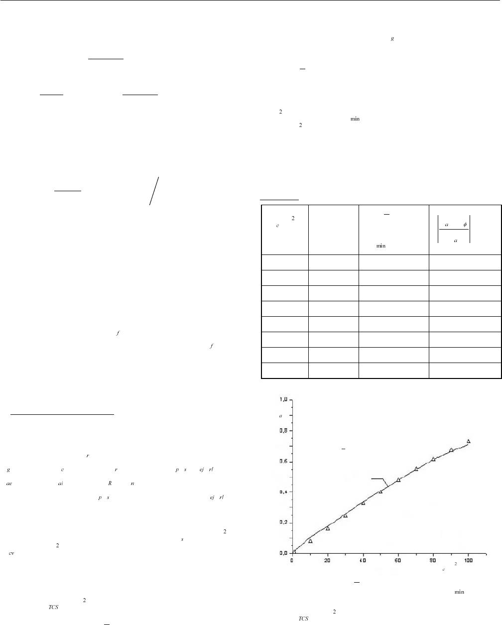
The
chartf −− φ prediction for the annual solar fraction
is compared with the numerical predictions of the present
simulation. The best fit for
a
f , for collector areas up to
80m is found for T = 77°C. It should be pointed out
that
80m is around the optimum economical area for the
solar assisted ejector cooling system as reported in [4]. The
numerical results for
a
f is shown in Table 1 while the
plots of
a
f for the best fit is shown in Fig. 2.
TABLE 1
(m )A
a
f
(present
work)
f chartφ−−
T = 77°C
100
ff
f
−
×
10 0.1029 0.07881 23.4110
20 0.1783 0.1606 9.92709
30 0.257 0.2424 5.68093
40 0.3352 0.3239 3.37112
50 0.4088 0.4013 1.83464
60 0.4788 0.4771 0.35505
70 0.5471 0.5496 0.45695
80 0.6113 0.6146 0.53983
present results
chartf −−φ
f
)m(A
(Δ)
Fig. 2: Plots of
chartf −− φ results for T = 77°C
against results for the annual fraction
a
f for
3mA = .