Van Harmelen F., Lifschitz V., Porter B. Handbook of Knowledge Representation
Подождите немного. Документ загружается.

472 11. Bayesian Networks
In fact, any independence statement derived this way can be read off the Bayesian
network structure using a graphical criterion known as d-separation [166, 35, 64].In
particular, we say that variables X are d-separated from variables Y by variables Z if
every (undirected) path from a node in X to a node in Y is blocked by Z. A path is
blocked by Z if it has a sequential or divergent node in Z, or if it has a convergent
node that is not in Z nor any of its descendants are in Z. Whether a node Z ∈ Z is se-
quential, divergent, or convergent depends on the way it appears on the path: → Z →
is sequential, ← Z → is divergent, and → Z ← is convergent. There are a number of
important facts about the d-separation test. First, it can be implemented in polynomial
time. Second, it is sound and complete with respect to the graphoid axioms. That is, X
and Y are d-separated by Z in DAG G if and only if the graphoid axioms can be used
to show that X and Y are independent given Z.
There are secondary structures that one can build from a Bayesian network which
can also be used to derive independence statements that hold in the distribution in-
duced by the network. In particular, the moral graph G
m
of a Bayesian network is an
undirected graph obtained by adding an undirected edge between any two nodes that
share a common child in DAG G, and then dropping the directionality of edges. If
variables X and Y are separated by variables Z in moral graph G
m
, we also have that
X and Y are independent given Z in any distribution induced by the corresponding
Bayesian network.
Another secondary structure that canbe used to derive independence statements for
a Bayesian network is the jointree [109]. This is a tree of clusters, where each cluster
is a set of variables in the Bayesian network, with two conditions. First, every family
(a node and its parents) in the Bayesian network must appear in some cluster. Second,
if a variable appears in two clusters, it must also appear in every cluster on the path
between them; see Fig. 11.4. Given a jointree for a Bayesian network (G, Θ),anytwo
clusters are independent given any cluster on the path connecting them [130]. One can
usually build multiple jointrees for a given Bayesian network, each revealing different
types of independence information. In general, the smaller the clusters of a jointree,
the more independence information it reveals. Jointrees play an important role in exact
inference algorithms as we shall discuss later.
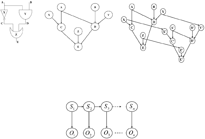
11.2.6 Dynamic Bayesian Networks
The dynamic Bayesian network (DBN) is a Bayesian network with a particular struc-
ture that deserves special attention [44, 119]. In particular, in a DBN, nodes are
partitioned into slices,0, 1,...,t, corresponding to different time points. Each slice
has the same set of nodes and the same set of inter-slice edges, except possibly for
the first slice which may have different edges. Moreover, intra-slice edges can only
cross from nodes in slice t to nodes in a following slice t + 1. Because of their recur-
rent structure, DBNs are usually specified using two slices only for t and t + 1; see
Fig. 11.2.
By restricting the structure of a DBN further at each time slice, one obtains more
specialized types of networks, some of which are common enough to be studied
outside the framework of Bayesian networks. Fig. 11.3 depicts one such restriction,
known as a Hidden Markov Model [160]. Here, variables S
i
typically represent un-
observable states of a dynamic system, and variables O
i
represent observable sensors
A. Darwiche 473
Figure 11.2: Two Bayesian network structures for a digital circuit. The one on the right is a DBN, repre-
senting the state of the circuit at two times steps. Here, variables A,...,E represent the state of wires in
the circuit, while variables X, Y, Z represent the health of corresponding gates.
Figure 11.3: A Bayesian network structure corresponding to a Hidden Markov Model.
that may provide information on the corresponding system state. HMMs are usually
studied as a special purpose model, and are equipped with three algorithms, known as
the forward–backward, Viterbi and Baum–Welch algorithms (see [138] for a descrip-
tion of these algorithms and example applications of HMMs). These are all special
cases of Bayesian network algorithms that we discuss in later sections.
Given the recurrent and potentially unbounded structure of DBNs (their size grows
with time), they present particular challenges and also special opportunities for in-
ference algorithms. They also admit a more refined class of queries than general
Bayesian networks. Hence, it is not uncommon to use specialized inference algorithms
for DBNs, instead of applying general purpose algorithms that one may use for arbi-
trary Bayesian networks. We will see examples of such algorithms in the following
sections.
11.3 Exact Inference
Given a Bayesian (G, Θ) over variables X, which induces a probability distribution
Pr, one can pose a number of fundamental queries with respect to the distribution Pr:
• Most Probable Explanation (MPE): What’s the most likely instantiation of net-
work variables X, given some evidence e?
MPE (e) = argmax
x
Pr(x, e).

474 11. Bayesian Networks
• Probability of Evidence (PR): What’s the probability of evidence e,Pr(e)?Re-
lated to this query is Posterior Marginals: What’s the conditional probability
Pr(X|e) for every variable X in the network
3
?
• Maximum a Posteriori Hypothesis (MAP): What’s the most likely instantiation
of some network variables M, given some evidence e?
MAP(e, M) = argmax
m
Pr(m, e).
These problems are all difficult. In particular, the decision version of MPE, PR, and
MAP, are known to be NP-complete, PP-complete and NP
PP
-complete, respectively
[32, 158, 145, 123]. We will discuss exact algorithms for answering these queries
in this section, and then discuss approximate algorithms in Section 11.4.Westart
in Section 11.3.1 with a class of algorithms known as structure-based as their com-
plexity is only a function of the network topology. We then discuss in Section 11.3.2
refinements of these algorithms that can exploit local structure in network parameters,
leading to a complexity which is both a function of network topology and parame-
ters. Section 11.3.3 discusses a class of algorithms based on search, specialized for
MAP and MPE problems. Section 11.3.4 discusses an orthogonal class of methods for
compiling Bayesian networks, and Section 11.3.5 discusses the technique of reducing
exact probabilistic reasoning to logical inference.
It should noted here that by evidence, we mean a variable instantiation e of some
network variables E. In general, one can define evidence as an arbitrary event α, yet
most of the algorithms we shall discuss assume the more specific interpretation of ev-
idence. These algorithms can be extended to handle more general notions of evidence
as discussed in Section 11.3.6, which discusses a variety of additional extensions to
inference algorithms.
11.3.1 Structure-Based Algorithms
When discussing inference algorithms, it is quite helpful to view the distribution in-
duced by a Bayesian network as a product of factors, where a factor f(X) is simply a
mapping from instantiations x of variables X to real numbers. Hence, each CPT Θ
X|U
of a Bayesian network is a factor over variables XU;seeFig. 11.1. The product of two
factors f(X) and f(Y) is another factor over variables Z = X ∪ Y: f(z) = f(x)f (y)
where z ∼ x and z ∼ y.
4
The distribution induced by a Bayesian network (G, Θ)
can then be expressed as a product of its CPTs (factors) and the inference problem in
Bayesian networks can then be formulated as follows. We are given a function f(X)
(i.e., probability distribution) expressed as a product of factors f
1
(X
1
),...,f
n
(X
n
)
and our goal is to answer questions about the function f(X) without necessarily com-
puting the explicit product of these factors.
We will next describe three computational paradigms for exact inference in
Bayesian networks, which share the same computational guarantees. In particular, all
methods can solve the PR and MPE problems in time and space which is exponential
3
From a complexity viewpoint, all posterior marginals can be computed using a number of PR queries
that is linear in the number of network variables.
4
Recall, that ∼ represents the compatibility relation among variable instantiations.
A. Darwiche 475
only in the network treewidth [8, 144]. Moreover, all can solve the MAP problem ex-
ponential only in the network constrained treewidth [123]. Treewidth (and constrained
treewidth) are functions of the network topology, measuring the extent to which a net-
work resembles a tree. A more formal definition will be given later.
Inference by variable elimination
The first inference paradigm we shall discuss is based on the influential concept
of variable elimination [153, 181, 45]. Given a function f(X) in factored form,
$
n
i=1
f
i
(X
i
), and some corresponding query, the method will eliminate a variable
X from this function to produce another function f
(X − X), while ensuring that the
new function is as good as the old function as far as answering the query of interest.
The idea is then to keep eliminating variables one at a time, until we can extract the
answer we want from the result. The key insight here is that when eliminating a vari-
able, we will only need to multiply factors that mention the eliminated variable. The
order in which variables are eliminated is therefore important as far as complexity is
concerned, as it dictates the extent to which the function can be kept in factored form.
The specific method for eliminating a variable depends on the query at hand. In
particular, if the goal is to solve PR, then we eliminate variables by summing them
out. If we are solving the MPE problem, we eliminate variables by maxing them out.
If we are solving MAP, we will have to perform both types of elimination. To sum out
a variable X from factor f(X) is to produce another factor over variables Y = X− X,
denoted
X
f , where (
X
f)(y) =
x
f(y,x). To max out variable X is similar:
(max
X
f)(y) = max
x
f(y,x). Note that summing out variables is commutative and
so is maxing out variables. However, summing out and maxing out do not commute.
For a Bayesian network (G, Θ) over variables X, map variables M, and some evidence
e, inference by variable elimination is then a process of evaluating the following ex-
pressions:
• MPE:max
X
$
X
Θ
X|U
λ
X
.
• PR:
X
$
X
Θ
X|U
λ
X
.
• MAP:max
M
X−M
$
X
Θ
X|U
λ
X
.
Here, λ
X
is a factor over variable X, called an evidence indicator, used to capture
evidence e: λ
X
(x) = 1ifx is consistent with evidence e and λ
X
(x) = 0 otherwise.
Evaluatingthe above expressions leads to computing the probability of MPE, the prob-
ability of evidence, and the probability of MAP, respectively. Some extra bookkeeping
allows one to recover the identity of MPE and MAP [130, 45].
As mentioned earlier, the order in which variables are eliminated is critical for
the complexity of variable elimination algorithms. In fact, one can define the width
of an elimination order as one smaller than the size of the largest factor constructed
during the elimination process, where the size of a factor is the number of variables
over which it is defined. One can then show that variable elimination has a complexity
which is exponential only in the width of used elimination order. In fact, the treewidth
of a Bayesian network can be defined as the width of its best elimination order. Hence,
the time and space complexity of variable elimination is bounded by O(n exp(w)),
where n is the number of network variables (also number of initial factors), and w is

476 11. Bayesian Networks
Figure 11.4: A Bayesian network (left) and a corresponding jointree (right), with the network factors and
evidence indicators assigned to jointree clusters.
the width of used elimination order [45]. Note that w is lower bounded by the network
treewidth. Moreover, computing an optimal elimination order and network treewidth
are both known to be NP-hard [9].
Since summing out and maxing out do not commute, we must max out variables M
last when computing MAP. This means that not all variable orders are legitimate; only
those in which variables M come last are. The M-constrained treewidth of a Bayesian
network can then be defined as the width of its best elimination order having vari-
ables M last in the order. Solving MAP using variable elimination is then exponential
in the constrained treewidth [123].
Inference by tree clustering
Tree clustering is another algorithm for exact inference, which is also known as the
jointree algorithm [89, 105, 157]. There are different ways for deriving the jointree
algorithm, one of which treats the algorithm as a refined way of applying variable
elimination.
The idea is to organize the given set of factors into a tree structure, using a jointree
for the given Bayesian network. Fig. 11.4 depicts a Bayesian network, a corresponding
jointree, and assignment of thefactors to the jointreeclusters. We can then use the join-
tree structure to control the process of variable elimination as follows. We pick a leaf
cluster C
i
(having a single neighbor C
j
) in the jointree and then eliminate variables
that appear in that cluster but in no other jointree cluster. Given the jointree properties,
these variables are nothing but C
i
\ C
j
. Moreover, eliminating these variables requires
that we compute the product of all factors assigned to cluster C
i
and then eliminate
C
i
\ C
j
from the resulting factor. The result of this elimination is usually viewed as
a message sent from cluster C
i
to cluster C
j
. By the time we eliminate every cluster
but one, we would have projected the factored function on the variables of that clus-
ter (called the root). The basic insight of the jointree algorithm is that by choosing
different roots, we can project the factored function on every cluster in the jointree.
Moreover, some of the work we do in performing the elimination process towards one
root (saved as messages) can be reused when eliminating towards another root. In fact,
the amount of work that can be reused is such that we can project the function f on
all clusters in the jointree with time and space bounded by O(n exp(w)), where n is

A. Darwiche 477
the number of jointree clusters and w is the width of given jointree (size of its largest
cluster minus 1). This is indeed the main advantage of the jointree algorithm over the
basic variable elimination algorithm, which would need O(n
2
exp(w)) time and space
to obtain the same result. Interesting enough, if a network has treewidth w, then it
must have a jointree whose largest cluster has size w + 1. In fact, every jointree for
the network must have some cluster of size w + 1. Hence, another definition for the
treewidth of a Bayesian network is as the width of its best jointree (the one with the
smallest maximum cluster).
5
The classical description of a jointree algorithm is as follows (e.g., [83]). We first
construct a jointree for the given Bayesian network; assign each network CPT Θ
X|U
to
a cluster that contains XU; and then assign each evidence indicator λ
X
to a cluster that
contains X. Fig. 11.4 provides an example of this process. Given evidence e, a jointree
algorithm starts by setting evidence indicators according to given evidence. A cluster
is then selected as the root and message propagation proceeds in two phases, inward
and outward. In the inward phase, messages are passed toward the root. In the outward
phase, messages are passed away from the root. The inward phase is also known as the
collect or pull phase, and the outward phase is known as the distribute or push phase.
Cluster i sends a message to cluster j only when it has received messages from all
its other neighbors k. A message from cluster i to cluster j is a factor M
ij
defined as
follows:
M
i,j
=
C
i
\C
j
Φ
i
#
k=j
M
k,i
,
where Φ
i
is the product of factors and evidence indicators assigned to cluster i. Once
message propagation is finished, we have the following for each cluster i in the join-
tree:
Pr(C
i
, e) = Φ
i
#
k
M
k,i
.
Hence, we can compute the joint marginal for any subset of variables that is included
inacluster.
The above description corresponds to a version of the jointree algorithm known as
the Shenoy–Shafer architecture [157]. Another popular version of the algorithm is the
Hugin architecture [89]. The two versions differ in their space and time complexity
on arbitrary jointrees [106]. The jointree algorithm is quite versatile allowing even
more architectures (e.g., [122]), more complex types of queries (e.g., [91, 143, 34]),
including MAP and MPE, and a framework for time space tradeoffs [47].
Inference by conditioning
A third class of exact inference algorithms is based on the concept of conditioning
[129, 130, 39, 81, 162, 152, 37, 52]. The key concept here is that if we know the
value of a variable X in a Bayesian network, then we can remove edges outgoing
from X, modify the CPTs for children of X, and then perform inference equivalently
on the simplified network. If the value of variable X is not known, we can still ex-
ploit this idea by doing a case analysis on variable X, hence, instead of computing
5
Jointrees correspond to tree-decompositions [144] in the graph theoretic literature.
478 11. Bayesian Networks
Pr(e), we compute
x
Pr(e,x). This idea of conditioning can be exploited in different
ways. The first exploitation of this idea was in the context of loop-cutset conditioning
[129, 130, 11]. A loop-cutset for a Bayesian network is a set of variables C such that
removing edges outgoing from C will render the network a polytree: one in which
we have a single (undirected) path between any two nodes. Inference on polytree net-
works can indeed be performed in time and space linear in their size [129]. Hence,
by using the concept of conditioning, performing case analysis on a loop-cutset C,
one can reduce the query Pr(e) into a set of queries
c
Pr(e, c), each of which can be
answered in linear time and space using the polytree algorithm.
This algorithm has linear space complexity as one needs to only save modest in-
formation across the different cases. This is a very attractive feature compared to
algorithms based on elimination. The bottleneck for loop-cutset conditioning, how-
ever, is the size of cutset C since the time complexity of the algorithm is exponential
in this set. One can indeed construct networks which have a bounded treewidth, lead-
ing to linear time complexity by elimination algorithms, yet an unbounded loop-cutset.
A number of improvements have been proposed on loop-cutset conditioning (e.g., [39,
81, 162, 152, 37, 52]), yet only recursive conditioning [39] and its variants [10, 46]
have a treewidth-based complexity similar to elimination algorithms.
The basic idea behind recursive conditioning is to identify a cutset C that is not
necessarily a loop-cutset, but that can decompose a network N in two (or more) sub-
networks, say, N
l
c
and N
r
c
with corresponding distributions Pr
l
c
and Pr
r
c
for each
instantiation c of cutset C. In this case, we can write
Pr(e) =
c
Pr(e, c) =
c
Pr
l
c
(e
l
, c
l
)Pr
r
c
(e
r
, c
r
),
where e
l
/c
l
and e
r
/c
r
are parts of evidence/cutset pertaining to networks N
l
and N
r
,
respectively. The subqueries Pr
l
c
(e
l
, c
l
) and Pr
r
c
(e
r
, c
r
) can then be solved using the
same technique, recursively, by finding cutsets for the corresponding subnetworks N
l
c
and N
r
c
. This algorithm is typically driven by a structure known as a dtree, which is
a binary tree with its leaves corresponding to the network CPTs. Each dtree provides
a complete recursive decomposition over the corresponding network, with a cutset for
each level of the decomposition [39].
Given a dtree where each internal node T has children T
l
and T
r
, and each leaf
node has a CPT associated with it, recursive conditioning can then compute the prob-
ability of evidence e as follows:
rc(T , e) =
%
c
rc(T
l
, ec)rc(T
r
, ec), T is an internal node with cutset C;
ux∼e
θ
x|u
,Tis a leaf node with CPT Θ
X|U
.
Note that similar to loop-cutset conditioning, the above algorithm also has a linear
space complexity which is better than the space complexity of elimination algorithms.
Moreover, if the Bayesian network has treewidth w, there is then a dtree which is
both balanced and has cutsets whose sizes are bounded by w + 1. This means that the
above algorithm can run in O(n exp(w logn)) time and O(n) space. This is worse than
the time complexity of elimination algorithms, due to the log n factor, where n is the
number of network nodes.
A. Darwiche 479
A careful analysis of the above algorithm, however, reveals that it may make iden-
tical recursive calls in different parts of the recursion tree. By caching the value of a
recursive call rc(T , .), one can avoid evaluating the same recursive call multiple times.
In fact, if a network has a treewidth w, one can always construct a dtree on which
caching will reduce the running time from O(n exp(w logn)) to O(n exp(w)), while
bounding the space complexity by O(n exp(w)), which is identical to the complex-
ity of elimination algorithms. In principle, one can cache as many results as available
memory would allow, leading to a framework for trading off time and space [3], where
space complexity ranges from O(n) to O(n exp(w)), and time complexity ranges from
O(n exp(w logn)) to O(n exp(w)). Recursive conditioning can also be used to com-
pute multiple marginals [4], in addition to MAP and MPE queries [38], within the
same complexity discussed above.
We note here that the quality of a variable elimination order, a jointree and a dtree
can all be measured in terms of the notion of width, which is lower bounded by the
network treewidth. Moreover, the complexity of algorithms based on these structures
are all exponential only in the width of used structure. Polynomial time algorithms ex-
ists for converting between any of these structures, while preserving the corresponding
width, showing the equivalence of these methods with regards to their computational
complexity in terms of treewidth [42].
11.3.2 Inference with Local (Parametric) Structure
The computational complexity bounds given for elimination, clustering and condi-
tioning algorithms are based on the network topology, as captured by the notions
of treewidth and constrained treewidth. There are two interesting aspects of these
complexity bounds. First, they are independent of the particular parameters used to
quantify Bayesian networks. Second, they are both best-case and worst-case bounds
for the specific statements given for elimination and conditioning algorithms.
Given these results, only networks with reasonable treewidth are accessible to
these structure-based algorithms. One can provide refinements of both elimina-
tion/clustering and conditioning algorithms, however, that exploit the parametric struc-
ture of a Bayesian network, allowing them to solve some networks whose treewidth
can be quite large.
For elimination algorithms, the key is to adopt nontabular representations of
factors as initially suggested by [182] and developed further by other works (e.g.,
[134, 50, 80, 120]). Recall that a factor f(X ) over variables X is a mapping from in-
stantiations x of variables X to real numbers. The standard statements of elimination
algorithms assume that a factor f(X) is represented by a table that has one row of
each instantiation x. Hence, the size of factor f(X) is always exponential in the num-
ber of variables in X. This also dictates the complexity of factor operations, including
multiplication, summation and maximization. In the presence of parametric structure,
one can afford to use more structured representations of factors that need not be ex-
ponential in the variables over which they are defined. In fact, one can use any factor
representation as long as they provide corresponding implementations of the factor
operations of multiplication, summing out, and maxing out, which are used in the con-
text of elimination algorithms. One of the more effective structured representations of
factors is the algebraic decision diagram (ADD) [139, 80], which provides efficient
implementations of these operations.
480 11. Bayesian Networks
In the context of conditioning algorithms, local structure can be exploited at mul-
tiple levels. First, when considering the cases c of a cutset C, one can skip a case
c if it is logically inconsistent with the logical constraints implied by the network
parameters. This inconsistency can be detected by some efficient logic propagation
techniques that run in the background of conditioning algorithms [2]. Second, one
does not always need to instantiate all cutset variables before a network is discon-
nected or converted into a polytree, as some partial cutset instantiations may have the
same effect if we have context-specific independence [15, 25]. Third, local structure
in the form of equal network parameters within the same CPT will reduce the num-
ber of distinct subproblems that need to be solved by recursive conditioning, allowing
caching to be much more effective [25]. Considering various experimental results re-
ported in recent years, it appears that conditioningalgorithms have been more effective
in exploiting local structure, especially determinism, as compared to algorithms based
on variable eliminating (and, hence, clustering).
Network preprocessing can also be quite effective in the presence of local struc-
ture, especially determinism, and is orthogonal to the algorithms used afterwards. For
example, preprocessing has proven quite effective and critical for networks corre-
sponding to genetic linkage analysis, allowing exact inference on networks with very
high treewidth [2, 54, 55, 49]. A fundamental form of preprocessing is CPT decom-
position, in which one decomposes a CPT with local structure (e.g., [73]) into a series
of CPTs by introducing auxiliary variables [53, 167]. This decomposition can reduce
the treewidth of given network, allowing inference to be performed much more ef-
ficiently. The problem of finding an optimal CPT decomposition corresponds to the
problem of determining tensor rank [150], which is NP-hard [82]. Closed form solu-
tions are known, however, for CPTs with a particular local structure [150].
11.3.3 Solving MAP and MPE by Search
MAP and MPE queries are conceptually different from PR queries as they correspond
to optimization problems whose outcome is a variable instantiation instead of a prob-
ability. These queries admit a very effective class of algorithms based on branch and
bound search. For MPE, the search tree includes a leaf for each instantiation x of
nonevidence variables X, whose probability can be computed quite efficiently given
Eq. (11.3). Hence, the key to the success of these search algorithms is the use of
evaluation functions that can be applied to internal nodes in the search tree, which
correspond to partial variable instantiations i, to upper bound the probability of any
completion x of instantiation i. Using such an evaluation function, one can possibly
prune part of the search space, therefore, solving MPE without necessarily examining
the space of all variable instantiations. The most successful evaluation functions are
based on relaxations of the variable elimination algorithm, allowing one to eliminate a
variable without necessarily multiplying all factors that include the variable [95, 110].
These relaxations lead to a spectrum of evaluation functions, that can trade accuracy
with efficiency.
A similar idea can be applied to solving MAP, with a notable distinction. In MAP,
the search tree will be over the space of instantiations of a subset M of network vari-
ables. Moreover, each leaf node in the search tree will correspond to an instantiation m
in this case. Computing the probability of a partial instantiation m requires a PR query
A. Darwiche 481
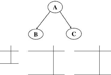
A θ
A
true 0.5
false 0.5
ABθ
B|A
true true 1
true false 0
false true 0
false false 1
ACθ
C|A
true true 0.8
true false 0.2
false true 0.2
false false 0.8
Figure 11.5: A Bayesian network.
though, which itself can be exponential in the network treewidth. Therefore, the suc-
cess of search-based algorithms for MAP depends on both the efficient evaluation of
leaf nodes in the search tree, and on evaluation functions for computing upper bounds
on the completion of partial variable instantiations [123, 121]. The most successful
evaluation function for MAP is based on a relaxation of the variable elimination algo-
rithm for computing MAP, allowing one to use any variable order instead of insisting
on a constrained variable order [121].
11.3.4 Compiling Bayesian Networks
The probability distribution induced by a Bayesian network can be compiled into an
arithmetic circuit, allowing various probabilistic queries to be answered in time linear
in the compiled circuit size [41]. The compilation time can be amortized over many
online queries, which can lead to extremely efficient online inference [25, 27].Com-
piling Bayesian networks is especially effective in the presence of local structure, as
the exploitation of local structure tends to incur some overhead that may not be justi-
fiable in the context of standard algorithms when the local structure is not excessive.
In the context of compilation, this overhead is incurred only once in the offline com-
pilation phase.
To expose the semantics of this compilation process, we first observe that the prob-
ability distribution induced by a Bayesian network, as given by Eq. (11.3), can be
expressed in a more general form:
(11.4)f =
x
#
λ
x
:x ∼ x
λ
x
#
θ
x|u
:xu∼ x
θ
x|u
,
where λ
x
is called an evidence indicator variable (we have one indicator λ
x
for each
variable X and value x). This form is known as the network polynomial and represents
the distribution as follows. Given any evidence e,letf(e) denotes the value of poly-
nomial f with each indicator variable λ
x
setto1ifx is consistent with evidence e and
set to 0 otherwise. It then follows that f(e) is the probability of evidence e. Following
is the polynomial for the network in Fig. 11.5:
f = λ
a
λ
b
λ
c
θ
a
θ
b|a
θ
c|a
+ λ
a
λ
b
λ
¯c
θ
a
θ
b|a
θ
¯c|a
+···λ
¯a
λ
¯
b
λ
¯c
θ
¯a
θ
¯
b|¯a
θ
¯c|¯a
.