Van Harmelen F., Lifschitz V., Porter B. Handbook of Knowledge Representation

Подождите немного. Документ загружается.

482 11. Bayesian Networks

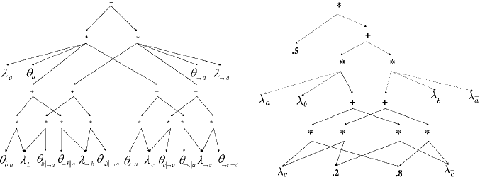
Figure 11.6: Two circuits for the Bayesian network in Fig. 11.5.

The network polynomial has an exponential number of terms, but can be factored

and represented more compactly usingan arithmetic circuit, which isa rooted, directed

acyclic graph whose leaf nodes are labeled with evidence indicators and network pa-

rameters, and internal nodes are labeled with multiplication and addition operations.

The size of an arithmetic circuit is measured by the number of edges that it contains.

Fig. 11.6 depicts an arithmetic circuit for the above network polynomial. This arith-

metic circuit is therefore a compilation of corresponding Bayesian network as it can

be used to compute the probability of any evidence e by evaluating the circuit while

setting the indicators to 1/0 depending on their consistency with evidence e. In fact,

the partial derivatives of this circuit with respect to indicators λ

and parameters θ

x|u

can all be computed in a single second pass on the circuit. Moreover, the values of

these derivatives can be used to immediately answer various probabilistic queries, in-

cluding the marginals over networks variables and families [41]. Hence, for a given

evidence, one can compute the probability of evidence and posterior marginals on all

network variables and families in two passes on the arithmetic circuit.

One can compile a Bayesian network using exact algorithms based on elimination

[26] or conditioning [25], by replacing their addition and multiplication operations

by corresponding operations for building the circuit. In fact, for jointree algorithms,

the arithmetic circuit can be generated directly from the jointree structure [124].One

can also generate these compilations by reducing the problem to logical inference

as discussed in the following section. If structure-based versions of elimination and

conditioning algorithms are used to compile Bayesian networks, the size of compiled

arithmetic circuits will be exponential in the network treewidth in the best case. If

one uses versions that exploit parametric structure, the resulting compilation may not

be lower bounded by treewidth [25, 27]. Fig. 11.6 depicts two arithmetic circuits for

the same network, the one on the right taking advantage of network parameters and

is therefore smaller than the one on the left, which is valid for any value of network

parameters.

11.3.5 Inference by Reduction to Logic

One of the more effective approaches for exact probabilistic inference in the presence

of local structure, especially determinism, is based on reducing the problem to one of

A. Darwiche 483

A Θ

0.1

0.9

ABΘ

B|A

0.1

0.9

0.2

0.8

ACΘ

C|A

0.1

0.9

0.2

0.8

Figure 11.7: The CPTs of Bayesian network with two edges A → B and A → C.

logical inference. The key technique is to encode the Bayesian network as a proposi-

tional theory in conjunctive normal form (CNF) and then apply algorithms for model

counting [147] or knowledge compilation to the resulting CNF [40]. The encoding can

be done in multiple ways [40, 147], yet we focus on one particular encoding [40] in

this section to illustrate the reduction technique.

We will now discuss the CNF encoding for the Bayesian network in Fig. 11.7.We

ﬁrst deﬁne the CNF variables which are in one-to-one correspondence with evidence

indicators and network parameters as deﬁned in Section 11.3.4, but treated as propo-

sitional variables in this case. The CNF  is then obtained by processing network

variables and CPTs, writing corresponding clauses as follows:

Variable A: λ

∨ λ

¬λ

∨¬λ

Variable B: λ

∨ λ

¬λ

∨¬λ

Variable C: λ

∨ λ

¬λ

∨¬λ

CPT for A: λ

⇔ θ

CPT for B: λ

∧ λ

⇔ θ

∧ λ

⇔ θ

∧ λ

⇔ θ

∧ λ

⇔ θ

CPT for C: λ

∧ λ

⇔ θ

∧ λ

⇔ θ

∧ λ

⇔ θ

∧ λ

⇔ θ

The clauses for variables are simply asserting that exactly one evidence indicator must

be true. The clauses for CPTs are establishing an equivalence between each network

parameter and its corresponding indicators. This resulting CNF has two important

properties. First, its size is linear in the network size. Second, its models are in one-to-

one correspondence with the instantiations of network variables. Table 11.2 illustrates

the variable instantiations and corresponding CNF models for the previous example.

We can now either apply a model counter to the CNF queries [147], or compile the

CNF to obtain an arithmetic circuit for the Bayesian network [40]. If we want to apply

a model counter to the CNF, we must ﬁrst assign weights to the CNF variables (hence,

we will be performing weighted model counting). All literals of the form λ

, ¬λ

and

¬θ

x|u

get weight 1, while literals of the form θ

x|u

get a weight equal to the value of

parameter θ

x|u

as deﬁned by the Bayesian network; see Table 11.2. To compute the

probability of any event α, all we need to do then is computed the weighted model

count of  ∧ α.

This reduction of probabilistic inference to logical inference is currently the most

effective technique for exploiting certain types of parametric structure, including de-

terminism and parameter equality. It also provides a very effective framework for

exploiting evidence computationally and for accommodating general types evidence

[25, 24, 147, 27].

484 11. Bayesian Networks

Table 11.2. Illustrating the models and corresponding weights of a CNF encod-

ing a Bayesian network

Network

instantiation

CNF

model

sets these CNF vars to

true and all others to false

Model weight

0.1 · 0.1 · 0.1 = 0.001

0.1 · 0.1 · 0.9 = 0.009

0.1 · 0.9 · 0.1 = 0.009

0.1 · 0.9 · 0.9 = 0.081

0.9 · 0.2 · 0.2 = 0.036

0.9 · 0.2 · 0.8 = 0.144

0.9 · 0.8 · 0.2 = 0.144

0.9 · 0.8 · 0.8 = 0.576

11.3.6 Additional Inference Techniques

We discuss in this section some additional inference techniques which can be crucial

in certain circumstances.

First, all of the methods discussed earlier are immediately applicable to DBNs.

However, the speciﬁc, recurrent structure of these networks calls for some special

attention. For example, PR queries can be further reﬁned depending on the location

of evidence and query variables within the network structure, leading to specialized

queries, such as monitoring. Here, the evidence is restricted to network slices t = 0,

...,t = i and the query variables are restricted to slice t = i. In such a case, and by

using restricted elimination orders, one can perform inference in space which is better

than linear in the network size [13, 97, 12]. This is important for DBNs as a linear

space complexity can be unpractical if we have too many slices.

Second, depending on the given evidence and query variables, a network can po-

tentially be pruned before inference is performed. In particular, one can always remove

edges outgoing from evidence variables [156]. One can also remove leaf nodes in the

network as long as they do not correspond to evidence or query variables [155].This

process of node removal can be repeated, possibly simplifying the network structure

considerably. More sophisticated pruning techniques are also possible [107].

Third, we have so far considered only simple evidence corresponding to the instan-

tiation e of some variables E. If evidence corresponds to a general event α, we can add

an auxiliary node X

to the network, making it a child of all variables U appearing

in α, setting the CPT Θ

based on α, and asserting evidence on X

[130].Amore

effective solution to this problem can be achieved in the context of approaches that

reduce the problem to logical inference. Here, we can simply add the event α to the

encoded CNF before we apply logical inference [147, 24]. Another type of evidence

we did not consider is soft evidence. This can be speciﬁed intwo forms. We can declare

that the evidence changes the probability of some variable X from Pr(X) to Pr



(X).

Or we can assert that the new evidence on X changes its odds by a given factor k,

known as the Bayes factor: O



(X)/O(X) = k. Both types of evidence can be handled

by adding an auxiliary child X

for node X, setting its CPT Θ

depending on the

strength of soft evidence, and ﬁnally simulating the soft evidence by hard evidence on

[130, 22].

A. Darwiche 485

11.4 Approximate Inference

All exact inference algorithms we have discussed for PR have a complexity which is

exponential in the network treewidth. Approximate inference algorithms are generally

not sensitive to treewidth, however, and can be quite efﬁcient regardless of the net-

work topology. The issue with these methods is related to the quality of answers the

compute, which for some algorithms is quite related to the amount of time budgeted

by the algorithm. We discuss two major classes of approximate inference algorithms

in this section. The ﬁrst and more classical class is based on sampling. The second and

more recent class of methods can be understood in terms of a reduction to optimization

problems. We note, however, that none of these algorithms offer general guarantees on

the quality of approximations they produce, which is not surprising since the problem

of approximating inference to any desired precision is known to be NP-hard [36].

11.4.1 Inference by Stochastic Sampling

Sampling from a probability distribution Pr(X) is a process of generating complete

instantiations x

,...,x

of variables X. A key property of a sampling process is its

consistency: generating samples x with a frequency that converges to their probabil-

ity Pr(x) as the number of samples approaches inﬁnity. By generating such consistent

samples, one can approximate the probability of some event α,Pr(α), in terms of the

fractions of samples that satisfy α,



Pr(α). This approximated probability will then

converge to the true probability as the number of samples reaches inﬁnity. Hence, the

precision of sampling methods will generally increase with the number of samples,

where the complexity of generating a sample is linear in the size of the network, and

is usually only weakly dependent on its topology.

Indeed, one can easily generate consistent samples from a distribution Pr that is

induced by a Bayesian network (G, Θ), using time that is linear in the network size to

generate each sample. This can be done by visiting the network nodes in topological

order, parents before children, choosing a value for each node X by sampling from the

distribution Pr(X|u) = Θ

X|u

, where u is the chosen values for X’s parents U.Thekey

question with sampling methods is therefore related to the speed of convergence (as

opposed to the speed of generating samples), which is usually affected by two major

factors: the query at hand (whether it has a low probability) and the speciﬁc network

parameters (whether they are extreme).

Consider, for example, approximating the query Pr(α|e) by approximating Pr(α, e )

and Pr(e) and then computing



Pr(α|e) =



Pr(α, e)/



Pr(e) according to the above sam-

pling method, known as logic sampling [76]. If the evidence e has a low probability,

the fraction of samples that satisfy e (and α, e for that matter) will be small, decreasing

exponentially in the number of variables instantiated by evidence e, and correspond-

ingly increasing the convergence time. The fundamental problem here is that we are

generating samples based on the original distribution Pr(X), where we ideally want to

generate samples based on the posterior distribution Pr(X|e), which can be shown to

be the optimal choice in a precise sense [28]. The problem, however, is that Pr(X|e)

is not readily available to sample from. Hence, more sophisticated approaches for

sampling attempt to sample from distributions that are meant to be close to Pr(X|e),

possibly changing the sampling distribution (also known as an importance function)

as the sampling process proceeds and more information is gained. This includes the

486 11. Bayesian Networks

methods of likelihood weighting [154, 63], self-importance sampling [154], heuristic

importance [154], adaptive importance sampling [28], and evidence pre-propagation

importance sampling (EPIS-BN) algorithm [179]. Likelihood weighing is perhaps the

simplest of these methods. It works by generating samples that are guaranteed to be

consistent with evidence e, by avoiding to sample values for variables E, always set-

ting them to e instead. It also assigns a weight of

e|u

:eu∼x

e|u

to each sample x.

Likelihood weighing will thenuse these weightedsamples for approximatingthe prob-

abilities of events. The current state of the art for sampling in Bayesian networks is

probably the EPIS-BN algorithm, which estimates the optimal importance function

using belief propagation (see Section 11.4.2) and then proceeds with sampling.

Another class of sampling methods is based on Markov Chain Monte Carlo

(MCMC) simulation [23, 128]. Procedurally, samples in MCMC are generated by ﬁrst

starting with a random sample x

that is consistent with evidence e.Asamplex

then generated based on sample x

i−1

by choosing a new value of some nonevidence

variable X by sampling from the distribution Pr(X|x

− X). This means that sam-

ples x

and x

i+1

will disagree on at most one variable. It also means that the sampling

distribution is potentially changed after each sample is generated. MCMC approxi-

mations will converge to the true probabilities if the network parameters are strictly

positive, yet the algorithm is known to suffer from convergence problems in case the

network parameters are extreme. Moreover, the sampling distribution of MCMC will

convergence to the optimal one if the network parameters satisfy some (ergodic) prop-

erties [178].

One specialized class of sampling methods, known as particle ﬁltering, deserves

particular attention at it applies to DBNs [93]. In this class, one generates particles

instead of samples, where a particle is an instantiation of the variables at a given time

slice t . One starts by a set of n particles for the initial time slice t = 0, and then

moves forward generating particles x

for time t based on the particles x

t−1

generated

for time t − 1. In particular, for each particle x

t−1

, we sample a particle x

based on

the distributions Pr(X

t−1

), in a fashion similar to logic sampling. The particles for

time t can then be used to approximate the probabilities of events corresponding to

that slice. As with other sampling algorithms, particle ﬁltering needs to deal with the

problem of unlikely evidence, a problem that is more exaggerated in the context of

DBNs as the evidence pertaining to slices t>iis generally not available when we

generate particles for times t  i. One simple approach for addressing this problem is

to resample the particles for time t based on the extent to which they are compatible

with the evidence e

at time t . In particular, we regenerate n particles for time t from

the original set based on the weight Pr(e

) assigned to each particle x

. The family

of particle ﬁltering algorithms include other proposals for addressing this problem.

11.4.2 Inference as Optimization

The second class of approximate inference algorithms for PR can be understood in

terms of reducing the problem of inference to one of optimization. This class includes

belief propagation (e.g., [130, 117, 56, 176]) and variational methods (e.g., [92, 85]).

Given a Bayesian network which induces a distribution Pr, variational methods

work by formulating approximate inference as an optimization problem. For example,

say we are interested in searching for an approximate distribution



Pr which is more

A. Darwiche 487

well behaved computationally than Pr. In particular, if Pr is induced by a Bayesian

network N which has a high treewidth, then



Pr could possibly be induced by another

network



N which has a manageable treewidth. Typically, one starts by choosing the

structure of network



N to meet certain computational constraints and then search

for a parametrization of



N that minimizes the KL-divergence between the original

distribution Pr and the approximate one



Pr [100]:





Pr(.|e), Pr(.|e)







Pr(w|e) log



Pr(w|e)

Ideally, we want parameters of network



N that minimize this KL-divergence, while

possibly satisfying additional constraints. Often, we can simply set to zero the par-

tial derivatives of KL(



Pr(.|e), Pr(.|e)) with respect to the parameters, and perform

an iterative search for parameters that solve the resulting system of equations. Note

that the KL-divergence is not symmetric. In fact, one would probably want to mini-

mize KL(Pr(.|e),



Pr(.|e)) instead, but this is not typically done due to computational

considerations (see [57, 114] for approaches using this divergence, based on local op-

timizations).

One of the simplest variational approaches is to choose a completely disconnected

network



N , leading to what is known as a mean-ﬁeld approximation [72]. Other vari-

ational approaches typically assume a particular structure of the approximate model,

such as chains [67], trees [57, 114], disconnected subnetworks [149, 72, 175],orjust

tractable substructures in general [173, 65]. These methods are typically phrased in

the more general setting of graphical models (which includes other representational

schemes, such as Markov Networks), but can typically be adapted to Bayesian net-

works as well. We should note here that the choice of approximate network



should at least permit one to evaluate the KL-divergence between



N and the orig-

inal network N efﬁciently. As mentioned earlier, such approaches seek minima of

the KL-divergence, but typically search for parameters where the partial derivatives

of the KL-divergence are zero, i.e., parameters that are stationary points of the KL-

divergence. In this sense, variational approaches can reduce the problem of inference

to one of optimization. Note that methods identifying stationary points, while con-

venient, only approximate the optimization problem since stationary points do not

necessarily represent minima of the KL-divergence, and even when they do, they do

not necessarily represent global minima.

Methods based on belief propagation [130, 117, 56] are similar in the sense that

they also can be understood as solving an optimization problem. However, this under-

standing is more recent and comes as an after fact of having discovered the ﬁrst belief

propagation algorithm, known as loopy belief propagation or iterative belief propa-

gation (IBP). In IBP, the approximate distribution



Pr is assumed to have a particular

factored form:

(11.5)



Pr(X|e) =

X∈X



Pr(XU|e)

U∈U



Pr(U|e)

where U ∈ U are parents of the nodeX in the original Bayesiannetwork N . This form

allows one to decompose the KL-divergence between the original and approximate

488 11. Bayesian Networks

distributions as follows:





Pr(.|e), Pr(.|e)







Pr(xu|e) log



Pr(xu|e)

u∼u



Pr(u|e)

−





Pr(xu|e) logθ

x|u

+ logPr(e).

This decomposition of the KL-divergence has important properties. First, the term

Pr(e) does not depend on the approximate distribution and can be ignored in the

optimization process. Second, all other terms are expressed as a function of the ap-

proximate marginals



Pr(xu|e) and



Pr(u|e), in addition to the original network parame-

ters θ

x|u

. In fact, IBP can be interpreted as searching for values of these approximate

marginals that correspond to stationary points of the KL-divergence: ones that set to

zero the partial derivatives of the divergence with respect to these marginals (under cer-

tain constraints). There is a key difference between the variational approaches based

on searching for parameters of approximate networks and those based on searching

for approximate marginals: The computed marginals may not actually correspond to

any particular distribution as the optimization problem solved does not include enough

constraints to ensure the global coherence of these marginals (only node marginals are

consistent, e.g.,



Pr(x|e) =





Pr(xu|e)).

The quality of approximations found by IBP depends on the extent to which the

original distribution can indeed be expressed as given in (11.5). If the original network

N has a polytree structure, the original distribution can be expressedas given in (11.5)

and the stationary point obtained by IBP corresponds to exact marginals. In fact, the

form given in (11.5) is not the only one that allows one to set up an optimization

problem as given above. In particular, any factored form that has the structure:

(11.6)



Pr(.|e) =



Pr(C|e)



Pr(S|e)

where C and S are sets of variables, will permit a similar decomposition of the KL-

divergence in terms of marginals



Pr(C|e) and



Pr(S|e). This leads to a more general

framework for approximate inference, known as generalized belief propagation [176].

Note, however, that this more general optimization problem is exponential in the sizes

of sets C and S. In fact, any distribution induced by a Bayesian network N can be ex-

pressed in the above form, if the sets C and S correspond to the clusters and separators

of a jointree for network N [130]. In that case, the stationary point of the optimization

problem will correspond to exact marginals, yet the size of the optimization problem

will be at least exponential in the network treewidth. The form in (11.6) can there-

fore be viewed as allowing one to trade the complexity of approximate inference with

the quality of computed approximations, with IBP and jointree factorizations being

two extreme cases on this spectrum. Methods for exploring this spectrum include

joingraphs (which generalize jointrees) [1, 48], region graphs [176, 169, 170], and

partially ordered sets (or posets) [111], which are structured methods for generating

factorizations with interesting properties.

The above optimization perspective on belief propagation algorithms is only meant

to expose the semantics behind these methods. In general, belief propagation algo-

rithms do not set up an explicit optimization problem as discussed above. Instead,

A. Darwiche 489

they operate by passing messages in a Bayesian network (as is done by IBP), a jo-

ingraph, or some other structure such as a region graph. For example, in a Bayesian

network, the message sent from a node X to its neighbor Y is based on the messages

that node X receives from its other neighbors Z = Y . Messages are typically initial-

ized according to some ﬁxed strategy, and then propagated according to some message

passing schedule. For example, one may update messages in parallel or sequentially

[168, 164]. Additional techniques are used to ﬁne tune the propagation method, in-

cluding message dampening [117, 78]. When message propagation converges (if it

does), the computed marginals are known to correspond to stationary points of the

KL-divergence as discussed above [176, 79]. There are methods that seek to optimize

the divergence directly, but they may be slow to converge [180, 171, 94, 174].

Statistical physics happens to be the source of inspiration for many of these meth-

ods and perspectives. In particular, we can reformulate the optimization of the KL-

divergence in terms of optimizing a variational free energy that approximates a free

energy (e.g., in thermodynamics). The free energy approximation corresponding to

IBP and Eq. (11.5) is often referred to as the Bethe free energy [176]. Other free en-

ergy approximations in physics that improve on, or generalize, the Bethe free energy

have indeed lent themselves to generalizing belief propagation. Among them is the

Kikuchi free energy [177], which led to region-based free energy approximations for

generalized belief propagation algorithms [176].

11.5 Constructing Bayesian Networks

Bayesian networks can be constructed in a variety of methods. Traditionally, Bayesian

networks have been constructed by knowledge engineers in collaboration with do-

main experts, mostly in the domain of medical diagnosis. In more recent applications,

Bayesian networks are typically synthesized from high level speciﬁcations, or learned

from data. We will review each of these approaches in the following sections.

11.5.1 Knowledge Engineering

The construction of Bayesian networks using traditional knowledge engineering tech-

niques has been most prevalent in medical reasoning, which also constitute some of

the ﬁrst signiﬁcant applications of Bayesian networks to real-world problems. Some

of the notable examples in this regard include: The Quick Medical Reference (QMR)

model [113] which was later reformulated as a Bayesian network model [159] that

covers more than 600 diseases and 4000 symptoms; the CPCS-PM network [137, 125],

which simulates patient scenarios in the medical ﬁeld of hepatobiliary disease; and the

MUNIN model for diagnosing neuromuscular disorders from data acquired by elec-

tromyographic (EMG) examinations [7, 5, 6], which covers 8 nerves and 6 muscles.

The construction of Bayesian networks using traditional knowledge engineering

techniques has been recently made more effective through progress on the subject of

sensitivity analysis: a form of analysis which focuseson understanding the relationship

between local network parameters and global conclusions drawn from the network

[102, 18, 90, 98, 19–21]. These results have lead to the creation of efﬁcient sensitivity

analysis tools which allow experts to assess the signiﬁcance of network parameters,

and to easily isolate problematic parameters when obtaining counterintuitive results to

posed queries.

490 11. Bayesian Networks

11.5.2 High-Level Speciﬁcations

The manual construction of large Bayesian networks can be laborious and error-prone.

In many domains, however, these networks tend to exhibit regular and repetitive struc-

tures, with the regularities manifesting themselves both at the level of individual CPTs

and at the level of network structure. We have already seen in Section 11.2.4 how reg-

ularities in a CPT can reduce the speciﬁcation of a large CPT to the speciﬁcation of a

few parameters. A similar situation can arise in the speciﬁcation of a whole Bayesian

network, allowing one to synthesize a large Bayesian network automatically from a

compact, high-level speciﬁcation that encodes probabilistic dependencies among net-

work nodes, in addition to network parameters.

This general knowledge-based model construction paradigm [172] has given rise

to many concrete high-level speciﬁcation frameworks, with a variety of representation

styles. All of these frameworks afford a certain degree of modularity, thus facilitat-

ing the adaptation of existing speciﬁcations to changing domains. A further beneﬁt

of high-level speciﬁcations lies in the fact that the smaller number of parameters they

contain can often be learned from empirical data with higher accuracy than the larger

number of parameters found in the full Bayesian network [59, 96]. We next describe

some fundamental paradigms for high-level representation languages, where we dis-

tinguish between two main paradigms: template-based and programming-based. It

must be acknowledged, however, that this simple distinction is hardly adequate to

account for the whole variety of existing representation languages.

Template-based representations

The prototypical example of template-based representations is the dynamic Bayesian

network described in Section 11.2.6. In this case, one speciﬁes a DBN having an ar-

bitrary number of slices using only two templates: one for the initial time slice, and

one for all subsequent slices. By further specifying the number of required slices t ,

a Bayesian network of arbitrary size can be compiled from the given templates and

temporal horizon t.

One can similarly specify other types of large Bayesian networks that are com-

posed of identical, recurring segments. In general, the template-based approach re-

quires two components for specifying a Bayesian network: a set of network templates

whose instantiation leads to network segments, and a speciﬁcation of which segments

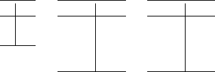
to generate and how to connect them together. Fig. 11.8 depicts three templates from

the domain of genetics, involving two classes of variables: genotypes (gt) and phe-

notypes (pt). Each template contains nodes of two kinds: nodes representing random

variables that are created by instantiating the template (solid circles, annotated with

CPTs), and nodes for input variables (dashed circles). Given these templates, to-

gether with a pedigree which enumerates particular individuals with their parental

relationships, one can then generate a concrete Bayesian network by instantiating one

genotype template and one phenotype template for each individual, and then con-

necting the resulting segments depending on the pedigree structure. The particular

genotype template instantiated for an individual will depend on whether the individual

is a founder (has no parents) in the pedigree.

The most basic type of template-based representations, such as the one in Fig. 11.8,

is quite rigid as all generated segments will have exactly the same structure. More

A. Darwiche 491

gt(X)

AA Aa aa

0.49 0.42 0.09

gt(X)

gt(p1(X)) gt(p2(X)) AA Aa aa

AA AA 1.0 0.0 0.0

AA Aa

0.5 0.5 0.0

... ...

... ... ...

aa aa

0.0 0.0 1.0

pt(X)

gt(X) affected not affected

AA 0.0 1.0

0.0 1.0

1.0 0.0

Figure 11.8: Templates for specifying a Bayesian network in the domain of genetics. The templates as-

sume three possible genotypes (AA, Aa, aa) and two possible phenotypes (affected, not affected).

sophisticated template-based representations add ﬂexibility to the speciﬁcation in var-

ious ways. Network fragments [103] allow nodes in a template to have an unspeci-

ﬁed number of parents. The CPT for such nodes must then be speciﬁed by generic

rules. Object oriented Bayesian networks [99] introduce abstract classes of network

templates that are deﬁned by their interface with other templates. Probabilistic re-

lational models enhance the template approach with elements of relational database

concepts [59, 66], by allowing one to deﬁne probabilities conditional on aggregates

of the values of an unspeciﬁed number of parents. For example, one might include

nodes life_expectancy(X) and age_at_death(X) into a template for individuals X, and

condition the distribution of life_expectancy(X) on the average value of the nodes

age_at_death(Y ) for all ancestors Y of X.

Programming-based representations

Frameworks in this group contain some of the earliest high-level representation lan-

guages. They use procedural or declarative speciﬁcations, which are not as directly

connected to graphical representations as template-based representations. Many are

based on logic programming languages [17, 132, 71, 118, 96]; others resemble func-

tional programming [86] or deductive database [69] languages. Compared to template-

based approaches, programming-based representations can sometimes allow more

modular and intuitive representations of high-level probabilistic knowledge. On the

other hand, the compilation of the Bayesian network from the high-level speciﬁcation