Vidakovic B. Statistics for Bioengineering Sciences: With Matlab and WinBugs Support

Подождите немного. Документ загружается.

288 8 Bayesian Approach to Inference

Table 8.1 Some conjugate pairs. Here X stands for a sample of size n, X

,..., X

. For func-

tional expressions of the densities and their moments refer to Chap. 5

Likelihood Prior Posterior

X |θ ∼N (θ,σ

) θ ∼N (µ, τ

) θ|X ∼N

+τ

X +

+τ

µ,

+τ

X |θ ∼B in(n,θ) θ ∼B e(α,β) θ|X ∼ B e(α +x, n −x +β)

|θ ∼P oi(θ) θ ∼G a(α, β) θ|X ∼G a(

+α, n +β).

|θ ∼N B(m,θ) θ ∼B e(α, β) θ|X ∼B e(α +mn, β +

)

∼G a(n/2,1/(2θ)) θ ∼ I G (α,β) θ|X ∼ I G (n/2+α, x/2 +β)

|θ ∼U (0, θ) θ ∼ P a(θ

,α) θ|X ∼P a(max{θ

, X

,..., X

},α +n)

|θ ∼N (µ,θ) θ ∼I G (α, β) θ|X ∼I G (α +1/2,β +(µ −X)

/2)

|θ ∼G a(ν, θ) θ ∼G a(α,β) θ|X ∼G a(α +ν,β +x)

for some constant C. The normalizing constant C is free of p and is equal to

(

)

m(x)B(α,β)

, where m(x) is the marginal distribution.

By inspecting the expression p

x+α−1

(1−p)

n−x+β−1

, it is easy to see that the

posterior density remains beta; it is

B e(x +α, n −x +β), and that normalizing

constant resolves to C

=1/B(x +α, n −x +β). From the equality of constants, it

follows that

m(x)B(α,β)

B(x +α, n −x +β)

and one can express the marginal

m(x)

B(x +α, n −x +β)

B(α, β)

which is known as a beta-binomial distribution.

8.4 Point Estimation

The posterior is the ultimate experimental summary for a Bayesian. The pos-

terior location measures (especially the mean) are of great importance. The

posterior mean is the most frequently used Bayes estimator for a parameter.

The posterior mode and median are alternative Bayes estimators.

8.4 Point Estimation 289

The posterior mode maximizes the posterior density in the same way that

the MLE maximizes the likelihood. When the posterior mode is used as an

estimator, it is called the maximum posterior (MAP) estimator. The MAP esti-

mator is popular in some Bayesian analyses in part because it is computation-

ally less demanding than the posterior mean or median. The reason for this is

simple; to ﬁnd a MAP, the posterior does not need to be fully speciﬁed because

argmax

π(θ|x) = argmax

f (x|θ)π(θ), that is, the product of the likelihood and

the prior as well as the posterior are maximized at the same point.

Example 8.5. Binomial-Beta Conjugate Pair. In Example 8.4 we argued

that for the likelihood X

|θ ∼B in(n,θ) and the prior θ ∼B e(α,β), the posterior

distribution is

B e(x +α, n − x +β). The Bayes estimator of θ is the expected

value of the posterior

α +x

(α +x)+(β +n −x)

α +x

α +β +n

This is actually a weighted average of the MLE, X /n, and the prior mean

α/(α +β),

α +β +n

α +β

α +β +n

α +β

Notice that, as n becomes large, the posterior mean approaches the MLE,

because the weight

n+α+β

tends to 1. On the other hand, when α or β or both

are large compared to n, the posterior mean is close to the prior mean. Because

of this interplay between n and prior parameters, the sum

α +β is called the

prior sample size, and it measures the inﬂuence of the prior as if additional

experimentation was performed and

α +β trials have been added. This is in

the spirit of Wilson’s proposal to “add two failures and two successes” to an

estimator of proportion (p. 254). Wilson’s estimator can be seen as a Bayes

estimator with a beta

B e(2, 2) prior.

Large

α indicates a small prior variance (for ﬁxed β, the variance of

B e(α, β) is proportional to 1/α

) and the prior is concentrated about its mean.

In general, the posterior mean will fall between the MLE and the prior

mean. This was demonstrated in Example 8.1. As another example, suppose

we ﬂipped a coin four times and tails showed up on all four occasions. We are

interested in estimating the probability of showing heads,

θ, in a Bayesian

fashion. If the prior is

U (0, 1), the posterior is proportional to θ

(1−θ)

, which

is a beta

B e(1, 5). The posterior mean shrinks the MLE toward the expected

value of the prior (1/2) to get

= 1/(1 +5) = 1/6, which is a more reasonable

estimator of

θ than the MLE. Note that the 3/n rule produces a conﬁdence

interval for p of [0,3/4], which is too wide to be useful (Sect. 7.4.4).

290 8 Bayesian Approach to Inference

Example 8.6. Uniform/Pareto Model. In Example 7.5 we had the observa-

tions X

=2, X

=5, X

=0.5, and X

=3 from a uniform U (0,θ) distribution.

We are interested in estimating

θ in a Bayesian fashion. Let the prior on θ

be Pareto P a(θ

,α) for θ

= 6 and α = 2. Then the posterior is also Pareto

P a(θ

∗

,α

∗

) with θ

∗

= max{θ

, X

(n)

} = max{6,5} = 6, and α

∗

= α +n = 2 +4 = 6.

The posterior mean is

∗

−1

=36/5 =7.2, and the median is θ

∗

·2

1/α

∗

=6 ·2

1/6

6.7348.

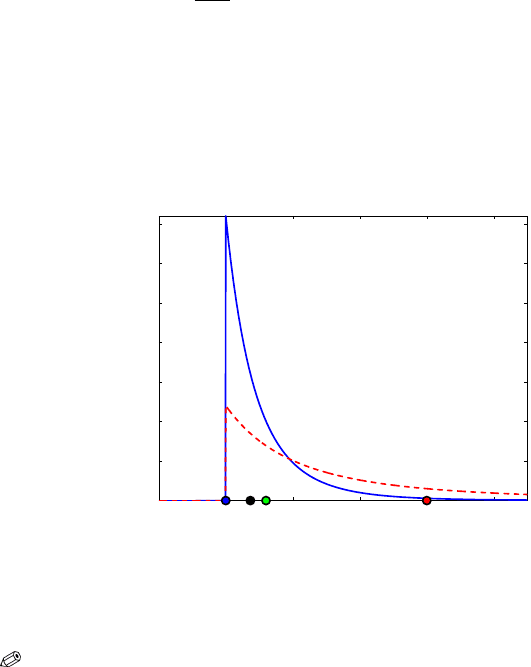
Figure 8.3 shows the prior (dashed red line) with the prior mean as a

red dot. After observing X

,... , X

, the posterior mode did not change since

the elicited

= 6 was larger than max X

= 5. However, the posterior has a

smaller variance than the prior. The posterior mean is shown as a green dot,

the posterior median as a black dot, and the posterior (and prior) mode as a

blue dot.

4 6 8 10 12 14

Fig. 8.3 Pareto P a(6, 2) prior (dashed red line) and P a(6,6) posterior (solid blue line). The

red dot is the prior mean, the green dot is the posterior mean, the black dot is the posterior

median, and the blue dot is the posterior (and prior) mode.

8.5 Prior Elicitation

Prior distributions are carriers of prior information that is coherently incorpo-

rated via Bayes’ theorem into an inference. At the same time, parameters are

unobservable, and prior speciﬁcation is subjective in nature. The subjectivity

of specifying the prior is a fundamental criticism of the Bayesian approach.

Being subjective does not mean that the approach is nonscientiﬁc, as critics

8.5 Prior Elicitation 291

of Bayesian statistics often insinuate. On the contrary, vast amounts of scien-

tiﬁc information coming from theoretical and physical models, previous exper-

iments, and expert reports guides the speciﬁcation of priors and merges such

information with the data for better inference.

In arguing about the importance of priors in Bayesian inference, Garth-

white and Dickey (1991) state that “expert personal opinion is of great poten-

tial value and can be used more efﬁciently, communicated more accurately,

and judged more critically if it is expressed as a probability distribution.”

In the last several decades Bayesian research has also focused on priors

that were noninformative and robust; this was in response to criticism that

results of Bayesian inference could be sensitive to the choice of a prior.

For instance, in Examples 8.4 and 8.5 we saw that beta distributions are

an appropriate family of priors for parameters supported in the interval [0,1],

such as a population proportion. It turns out that the beta family can express

a wide range of prior information. For example, if the mean

µ and variance

for a beta prior are elicited by an expert, then the parameters (a, b) can be

determined by solving

µ = a/(a+b) and σ

=ab/[(a+b)

(a +b +1)] with respect

to a and b:

=µ

µ(1 −µ)

−1

, and b =(1 −µ)

µ(1 −µ)

−1

. (8.4)

If a and b are not too small, the shape of a beta prior resembles a normal

distribution and the bounds [

µ−2σ, µ+2σ] can be used to describe the range of

likely parameters. For example, an expert’s claim that a proportion is unlikely

to be higher than 90% can be expressed as

µ +2σ =0.9.

In the same context of estimating the proportion, Berry and Stangl (1996)

suggest a somewhat different procedure:

(i) Elicit the probability of success in the ﬁrst trial, p

, and match it to the

prior mean

α/(α +β).

(ii) Given that the ﬁrst trial results in success, the posterior mean is

α+1

α+β+1

Match this ratio with the elicited probability of success in a second trial, p

conditional upon the ﬁrst trial’s resulting in success. Thus, a system

α +β

and p

α +1

α +β +1

is obtained that solves to

α =

(1 − p

)

− p

and β =

(1 − p

)(1 − p

)

− p

. (8.5)

See Exercise 8.12 for an application.

If one has no prior information, many noninformative choices are possible

such as invariant priors, Jeffreys’ priors, default priors, reference priors, and

intrinsic priors, among others. Informally speaking, a noninformative prior

292 8 Bayesian Approach to Inference

is one which is dominated by the likelihood, or that is “ﬂat” relative to the

likelihood.

Popular noninformative choices are the ﬂat prior

π(θ) = C for the location

parameter (mean) and

π(θ) =1/θ for the scale/rate parameter. A vague prior for

the proportion is p

−1

(1−p)

−1

, 0 < p <1. These priors are not proper probability

distributions, that is, they are not densities because their integrals are not

ﬁnite. However, Bayes’ theorem usually leads to posterior distributions that

are proper densities and on which Bayesian analysis can be carried out.

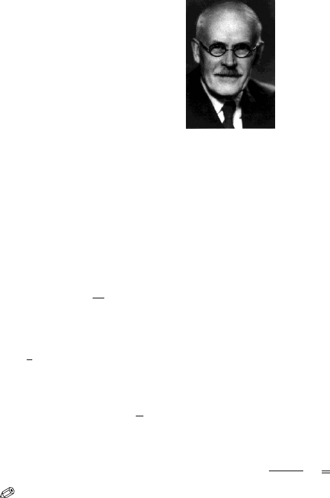
Fig. 8.4 Sir Harold Jeffreys, (1891–1989).

Jeffreys’ priors (named after Sir Harold Jeffreys, Fig. 8.4) are obtained

from a particular functional of a density (called Fisher information), and they

are also examples of vague and noninformative priors. For a binomial pro-

portion Jeffreys’ prior is proportional to p

−1/2

(1 − p)

−1/2

, while for the rate of

exponential distribution

λ Jeffreys’ prior is proportional to 1/λ. For a normal

distribution, Jeffreys’ prior on the mean is ﬂat, while for the variance

it is

proportional to

Example 8.7. If X

= 1.7, X

= 0.6, and X

= 5.2 come from an exponential

distribution with a rate parameter

λ, ﬁnd the Bayes estimator if the prior on

λ is

The likelihood is

−λ

and the posterior is proportional to

×λ

−λ

=λ

3−1

−λ

which is recognized as gamma

G a

. The Bayes estimator, as a mean

of this posterior, coincides with the MLE,

λ =

=1/2.5 =0.4.

An applied approach to prior selection was taken by Spiegelhalter et al.

(1994) in the context of biomedical inference and clinical trials. They recom-

mended a community of priors elicited from a large group of experts. A crude

classiﬁcation of community priors is as follows.

8.6 Bayesian Computation and Use of WinBUGS 293

(i) Vague priors – noninformative priors, in many cases leading to posterior

distributions proportional to the likelihood.

(ii) Skeptical priors – reﬂecting the opinion of a clinician unenthusiastic

about the new therapy, drug, device, or procedure. This may be a prior of a

regulatory agency.

(iii) Enthusiastic or clinical priors – reﬂecting the opinion of the proponents

of the clinical trial, centered around the notion that a new therapy, drug, de-

vice, or procedure is superior. This may be the prior of the industry involved

or clinicians running the trial.

For example, the use of a skeptical prior when testing for the superiority

of a new treatment would be a conservative approach. In equivalence tests,

both skeptical and enthusiastic priors may be used. The superiority of a new

treatment should be judged by a skeptical prior, while the superiority of the

old treatment should be judged by an enthusiastic prior.

8.6 Bayesian Computation and Use of WinBUGS

If the selection of an adequate prior is the major conceptual and modeling

challenge of Bayesian analysis, the major implementational challenge is com-

putation. When the model deviates from the conjugate structure, ﬁnding the

posterior distribution and the Bayes rule is all but simple. A closed-form solu-

tion is more the exception than the rule, and even for such exceptions, lucky

mathematical coincidences, convenient mixtures, and other tricks are needed

to uncover the explicit expression.

If classical statistics relies on optimization, Bayesian statistics relies on

integration. The marginal needed to normalize the product f (x

|θ)π(θ) is an

integral

m(x)

f (x|θ)π(θ)dθ,

while the Bayes estimator of h(

θ) is a ratio of integrals,

(x) =

h(θ)π(θ|x)dθ =

h(θ)f (x|θ)π(θ)dθ

f (x|θ)π(θ)dθ

The difﬁculties in calculating the above Bayes rule derive from the facts

that (i) the posterior may not be representable in a ﬁnite form and (ii) the in-

tegral of h(

θ) does not have a closed form even when the posterior distribution

is explicit.

The last two decades of research in Bayesian statistics has contributed to

broadening the scope of Bayesian models. Models that could not be handled

before by a computer are now routinely solved. This is done by Markov chain

294 8 Bayesian Approach to Inference

Monte Carlo (MCMC) methods, and their introduction to the ﬁeld of statistics

revolutionized Bayesian statistics.

The MCMC methodology was ﬁrst applied in statistical physics (Metropo-

lis et al., 1953). Work by Gelfand and Smith (1990) focused on applications of

MCMC to Bayesian models. The principle of MCMC is simple: One designs a

Markov chain that samples from the target distribution. By simulating long

runs of such a Markov chain, the target distribution can be well approximated.

Various strategies for constructing appropriate Markov chains that simulate

the desired distribution are possible: Metropolis–Hastings, Gibbs sampler,

slice sampling, perfect sampling, and many specialized techniques. These are

beyond the scope of this text, and the interested reader is directed to Robert

(2001), Robert and Casella (2004), and Chen et al. (2000) for an overview and

a comprehensive treatment.

In the examples that follow we will use WinBUGS for doing Bayesian infer-

ence when the models are not conjugate. Chapter 19 gives a brief introduction

to the front end of WinBUGS. Three volumes of examples are a standard addi-

tion to the software; in the Examples menu of WinBUGS, see Spiegelhalter et

al. (1996). It is recommended that you go over some of those examples in detail

because they illustrate the functionality and modeling power of WinBUGS. A

wealth of examples on Bayesian modeling strategies using WinBUGS can be

found in the monographs of Congdon (2001, 2003, 2005) and Ntzoufras (2009).

The following example is a WinBUGS solution of Example 8.2.

Example 8.8. Jeremy’s IQ in WinBUGS. We will calculate a Bayes estima-

tor for Jeremy’s true IQ,

θ, using simulations in WinBUGS. Recall that the

model was X

∼ N (θ,80) and θ ∼ N (100,120). WinBUGS uses precision in-

stead of variance to parameterize the normal distribution. Precision is sim-

ply the reciprocal of the variance, and in this example, the precisions are

1/120

= 0.00833 for the prior and 1/80 = 0.0125 for the likelihood. The Win-

BUGS code is as follows:

Jeremy in WinBUGS

model{

x ~ dnorm( theta, 0.0125)

theta ~ dnorm( 110, 0.008333333)

}

DATA

list(x=98)

INITS

list(theta=100)

Here is the summary of the MCMC output. The Bayes estimator for

rounded to 102.8. It is obtained as a mean of the simulated sample from the

posterior.

mean sd MC error val2.5pc median val97.5pc start sample

theta 102.8 6.943 0.01991 89.18 102.8 116.4 1001 100000

8.6 Bayesian Computation and Use of WinBUGS 295

Because this is a conjugate normal/normal model, the exact posterior dis-

tribution,

N (102.8,48), was easy to ﬁnd, (Example 8.2). Note that in these

simulations, the MCMC approximation, when rounded, coincides with the ex-

act posterior mean. The MCMC variance of

θ is 6.943

≈ 48.2, which is close

to the exact posterior variance of 48.

Another widely used conjugate pair is Poisson–gamma pair.

Example 8.9. Poisson–Gamma Conjugate Pair. Let X

,... , X

, given θ are

Poisson

P oi(θ) with probability mass function

f (x

|θ) =

−θ

and

θ ∼G (α,β) is given by π(θ) ∝θ

α−1

−βθ

. Then

π(θ|X

,... , X

) =π(θ|

) ∝θ

+α−1

−(n+β)θ

which is

G (

+α, n +β). The mean is E(θ|X ) =(

+α)/(n +β), and it can

be represented as a weighted average of the MLE and the prior mean:

Eθ|X =

n +β

Let us apply the above equation in a speciﬁc example. Let a rare disease

have an incidence of X cases per 100,000 people, where X is modeled as Pois-

son, X

|λ ∼ P oi(λ), where λ is the rate parameter. Assume that for different

cohorts of 100,000 subjects, the following incidences are observed: X

= 2,

= 0, X

= 4, X

= 0, X

= 1, X

= 3, and X

= 2. The ex-

perts indicate that

λ should be close to 2 and our prior is λ ∼ G a(0.2,0.1). We

matched the mean, since for a gamma distribution the mean is 0.2/0.1

=2 but

the variance 0.2/0.1

= 20 is quite large, thereby expressing our uncertainty.

By setting the hyperparameters to 0.02 and 0.01, for example, the variance of

the gamma prior would be even larger. The MLE of

λ is

mle

= X = 3/2. The

Bayes estimator is

8 +0.1

3/2

0.1

8 +0.1

=1.5062.

Note that since the prior was not informative, the Bayes estimator is quite

close to the MLE.

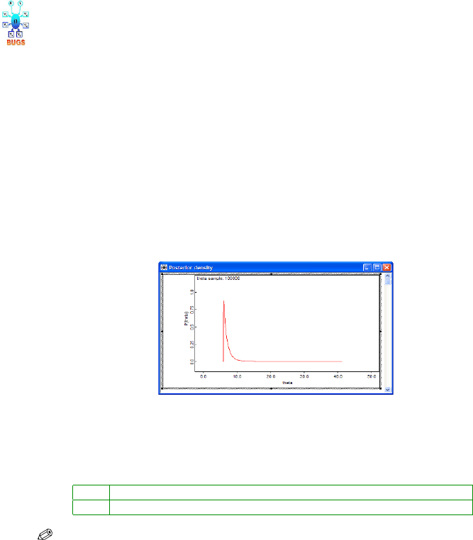
Example 8.10. Uniform/Pareto Model in WinBUGS. In Example 8.6 we

found that a posterior distribution of

θ, in a uniform U (0,θ ) model with a

Pareto

P a(6,2) prior, was Pareto P a(6,6). From the posterior we found the

mean, median, and mode to be 7.2, 6.7348, and 6, respectively. These are rea-

sonable estimators of

θ as location measures of the posterior.

296 8 Bayesian Approach to Inference

Uniform with Pareto in WinBUGS

model{

for (i in 1:n){

x[i] ~ dunif(0, theta);

}

theta ~ dpar(2,6)

}

DATA

list(n=4, x = c(2, 5, 0.5, 3) )

INITS

list(theta= 7)

Here is the summary of the WinBUGS output. The posterior mean was

found to be 7.196 and the median 6.736. Apparently, the mode of the posterior

was 6, as is evident from Fig. 8.5. These approximations are close to the exact

values found in Example 8.6.

Fig. 8.5 Output from Inference>Samples>density shows MCMC approximation to the

posterior distribution.

mean sd MC error val2.5pc median val97.5pc start sample

theta 7.196 1.454 0.004906 6.025 6.736 11.03 1001 100000

8.6.1 Zero Tricks in WinBUGS

Although the list of built-in distributions for specifying the likelihood or the

prior in WinBUGS is rich (p. 742), sometimes we encounter densities that are

not on the list.

How do we set the likelihood for a density that is not built into WinBUGS?

There are several ways, the most popular of which is the so-called zero

trick. Let f be an arbitrary model and

=log f (x

|θ) the log-likelihood for the

ith observation. Then

8.6 Bayesian Computation and Use of WinBUGS 297

i=1

f (x

|θ) =

i=1

(−`

)

−(−`

)

i=1

P oi(0,−`

The WinBUGS code for a zero trick can be written as follows.

Example 8.11. This example ﬁnds the Bayes estimator of parameter θ in a

Maxwell distribution with a density of f (x

|θ) =

3/2

−θx

, x ≥0, θ > 0.

The moment-matching estimator and the MLE have been discussed in Exam-

ple 7.4. For a sample of size n

=3, X

=1.4, X

=3.1, and X

=2.5 the MLE of

θ was

MLE

=0.5051. The same estimator was found by moment matching when

the second moment was matched. The Maxwell density is not implemented in

WinBUGS and we will use a zero trick instead.

#Estimation of Maxwell’s theta

#Using the zero trick

model{

for (i in 1:n){

zeros[i] <- 0

lambda[i] <- -llik[i] + 10000

zeros[i] ~ dpois(lambda[i])

llik[i] <- 1.5

log(theta)-0.5

theta

pow(x[i],2)

}

theta ~ dgamma(0.1, 0.1) #non-informative choice

}

DATA

list(n=3, x=c(1.4, 3.1, 2.5))

INITS

list(theta=1)

mean sd MC error val2.5pc median val97.5pc start sample

theta 0.5115 0.2392 8.645E-4 0.1559 0.4748 1.079 1001 100000

Note that the Bayes estimator with respect to a noninformative prior

dgamma(0.1, 0.1) is 0.5115.

for (i in 1:n){

zeros[i] <- 0

lambda[i] <- -llik[i] + 10000

# Since lambda[i] needs to be positive as

# a Poisson rate, an arbitrary constant C

# can be added; here we added C = 10000.

zeros[i] ~ dpois(lambda[i])

llik[i] <- ... write the log-likelihood function here

}