Vidakovic B. Statistics for Bioengineering Sciences: With Matlab and WinBugs Support

Подождите немного. Документ загружается.

298 8 Bayesian Approach to Inference

8.7 Bayesian Interval Estimation: Credible Sets

The Bayesian term for an interval estimator of a parameter is credible set.

Naturally, the measure used to assess the credibility of an interval estimator

is the posterior distribution. Students learning concepts of classical conﬁdence

intervals often err by stating that “the probability that a particular conﬁdence

interval [L,U] contains parameter

θ is 1 −α.” The correct statement seems

more convoluted; one generates data from the underlying model many times

and, for each generated data set, calculates the conﬁdence interval. The pro-

portion of conﬁdence intervals covering the unknown parameter “tends to”

−α. The Bayesian interpretation of a credible set C is arguably more natural:

the probability of a parameter belonging to set C is 1

−α. A formal deﬁnition

follows.

Assume set C is a subset of parameter space

Θ. Then C is a credible set

with credibility (1

−α)100% if

P(θ ∈C|X ) =E(I(θ ∈C)|X ) =

π(θ|x)dθ ≥1 −α.

If the posterior is discrete, then the integral is a sum (using the counting mea-

sure) and

P(θ ∈ C|X ) =

∈C

π(θ

|x) ≥1 −α.

This is the deﬁnition of a (1

−α)100% credible set. For a ﬁxed posterior dis-

tribution and a (1

−α)100% “credibility,” a credible set is not unique. We will

consider two versions of credible sets: highest posterior density (HPD) and

equal-tail credible sets.

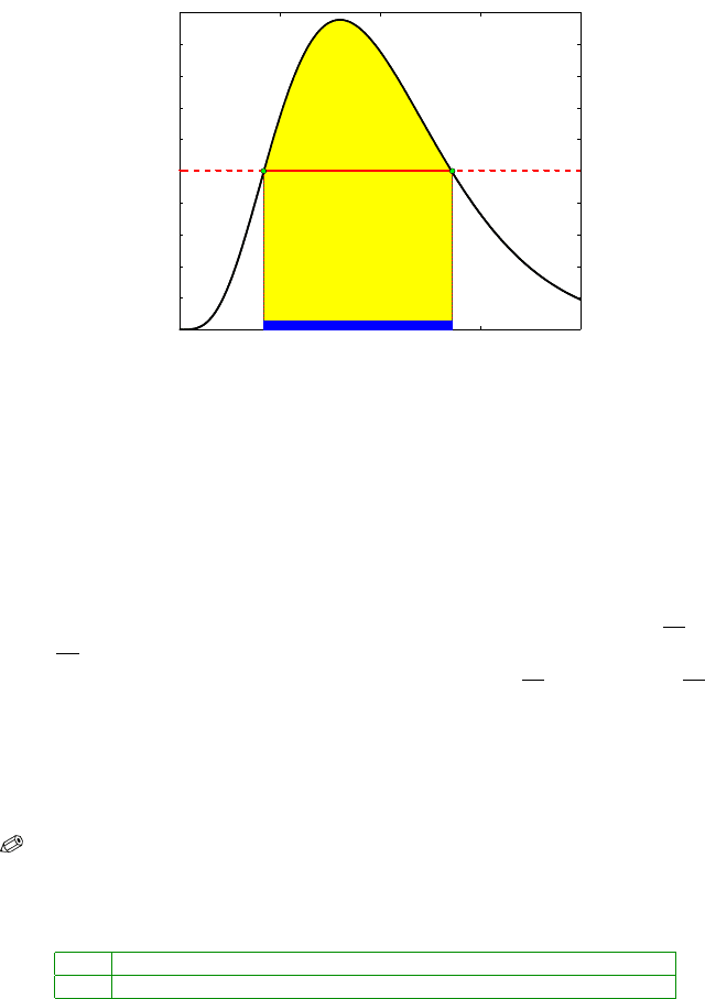
HPD Credible Sets. For a given credibility level (1

−α)100%, the shortest

credible set has obvious appeal. To minimize size, the sets should correspond

to the highest posterior probability density areas.

Deﬁnition 8.1. The (1

−α)100% HPD credible set for parameter θ is a set C,

a subset of parameter space

Θ of the form

={θ ∈Θ|π(θ|x) ≥ k(α)},

where k(

α) is the largest constant for which

P(θ ∈ C|X ) ≥1 −α.

Geometrically, if the posterior density is cut by a horizontal line at the

height k(

α), the credible set C is the projection on the θ-axis of the part of the

line that lies below the density (Fig. 8.6).

8.7 Bayesian Interval Estimation: Credible Sets 299

0 5 10 15 20

0.01

0.02

0.03

0.04

0.05

0.06

0.07

0.08

0.09

0.1

π(θ|x)

HPD (1 −α) × 100% Credible Set

1 − α

Fig. 8.6 Highest posterior density (HPD) (1−α)100% Credible Set (blue). The area in yellow

is 1

−α.

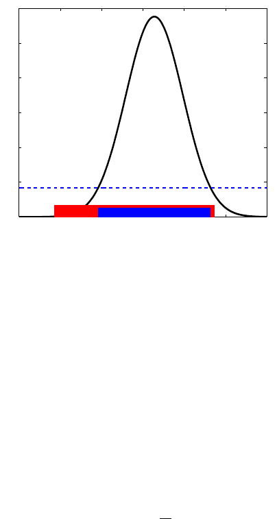
Example 8.12. Jeremy’s IQ, Continued. Recall Jeremy, the enthusiastic bio-

engineering student from Example 8.2 who used Bayesian inference in mod-

eling his IQ test scores. For a score of X he was using a

N (θ,80) likelihood,

while the prior on

θ was N (110,120). After the score of X = 98 was recorded,

the resulting posterior was normal

N (102.8,48).

Here, the MLE is

θ =98, and a 95% conﬁdence interval is [98−1.96

80, 98+

1.96

80] = [80.4692,115.5308]. The length of this interval is approx. 35. The

Bayesian counterparts are

θ =102.8, and [102.8−1.96

48, 102.8+1.96

48] =

[89.2207,116.3793]. The length of the 95% credible set is approx. 27. The

Bayesian interval is shorter because the posterior variance is smaller than

the likelihood variance; this is a consequence of the presence of prior informa-

tion. Figure 8.7 shows the credible set (in blue) and the conﬁdence interval (in

red).

From the WinBUGS output table in Jeremy’s IQ estimation example (p. 294)

the 95% credible set is [89.18,116.4].

mean sd MC error val2.5pc median val97.5pc start sample

theta 102.8 6.943 0.01991 89.18 102.8 116.4 1001 100000

Other posterior quantiles that lead to credible sets of different “credibil-

ity” levels can be speciﬁed in

Sample Monitor Tool under Inference>Samples in

WinBUGS. The credible sets from WinBUGS are HPD only if the posterior is

symmetric and unimodal.

Equal-Tail Credible Sets. HPD credible sets may be difﬁcult to ﬁnd

for asymmetric posterior distributions, such as gamma, Weibull, etc. Much

300 8 Bayesian Approach to Inference

70 80 90 100 110 120 130

0.01

0.02

0.03

0.04

0.05

0.06

Fig. 8.7 HPD 95% credible set based on a density of N (102.8, 48) (blue). The interval in

red is a 95% conﬁdence interval based on the observation X

= 98 and likelihood variance

=80.

simpler are equal-tail credible sets for which the tails have a probability of α/2

each for a credibility of 1

−α. An equal-tail credible set may not be the shortest

set, but to ﬁnd it we need only

α/2 and 1−α/2 quantiles of the posterior. These

two quantiles are the lower and upper bounds [L,U]:

−∞

π(θ|x) dθ =α/2,

∞

π(θ|x) dθ =1 −α/2.

Note that WinBUGS gives posterior quantiles from which one can directly es-

tablish several equal-tail credible sets (95%, 90%, 80%, and 50%) by selecting

appropriate pairs of percentiles in the

Sample Monitor Tool.

Example 8.13. Bayesian Amanita muscaria. Recall that in Example 7.8

(p. 251) observations were summarized by

X = 10.098 and s

=2.1702, which

are classical estimators of population parameters: mean

µ and variance σ

We also obtained the 95% conﬁdence interval for the population mean as

[9.6836,10.5124] and the 90% conﬁdence interval for the population variance

as [1.6074,3.1213].

By assuming noninformative priors for the mean and variance, we use

WinBUGS to ﬁnd Bayesian counterparts of the estimators and conﬁdence in-

tervals. As we pointed out, the mean is a location parameter, and noninforma-

tive priors should be “ﬂat.” WinBUGS allows for ﬂat priors,

mu∼dflat(), but

any prior with a large variance (or small precision) is a possibility. We take

a normal prior with a variance of 10,000. The inverse gamma distribution is

traditionally used for a prior on variance; thus, for precision as a reciprocal of

variance, the gamma prior is appropriate. As we discussed earlier, gamma dis-

tributions with small parameters will have a large variance, thereby making

8.8 Learning by Bayes’ Theorem 301

the prior vague/noninformative. We selected prec∼dgamma(0.001, 0.001) as a

noninformative choice. This prior is noninformative because it is essentially

ﬂat; its variance is 0.001/(0.001)

= 1000 (p. 166). The WinBUGS program is

simple:

model{

for ( i in 1:n ){

amuscaria[i] ~ dnorm( mu, prec )

}

mu ~ dnorm(0, 0.00001)

prec ~ dgamma(0.001, 0.001)

sig2 <- 1/prec

}

DATA

list(n=51,amuscaria=c(10,11,12,9,10,11,13,12,10,11,11,13,9,10,

9,10,8,12,10,11,9,10,7,11,8,9,11,11,10,12,10,8,7,11,12,

10,9,10,11,10,8,10,10,8,9,10,13,9,12,9,9) )

INITS

list( mu =0, prec = 1 )

In WinBUGS’ Sample Monitor Tool we asked for 2.5% and 97.5% poste-

rior percentiles, which gives a 95% credible set and 5% and 95% posterior

percentiles for the 90% credible set. The lower/upper bounds of the credible

sets are given in boldface and the sets are [9.684,10.51] for the mean and

[1.607,3.123] for the variance. The credible set for the mean is both HPD and

equal-tail, but the credible set for the variance is only an equal-tail.

mean sd MC error val2.5pc val5pc val95pc val97.5pc start sample

mu 10.1 0.2106 2.004E-4 9.684 9.752 10.44 10.51 1001 100000

prec 0.4608 0.09228 9.263E-5 0.2983 0.3202 0.6224 0.6588 1001 100000

sig2 2.261 0.472 4.716E-4 1.518 1.607 3.123 3.353 1001 100000

8.8 Learning by Bayes’ Theorem

We start with an example.

Example 8.14. Freireich et al. (1963) conducted a remission maintenance ther-

apy to compare 6-MP with placebo for prolonging the duration of remission in

leukemia. From 42 patients affected with acute leukemia, but in a state of

partial or complete remission, 21 pair was formed. One randomly selected pa-

tient from each pair was assigned the maintenance treatment 6-MP, while the

other patient received a placebo. Investigators monitored which patient stayed

in remission longer. If that was a patient from the 6-MP treatment arm, this

was recorded as a “success” (S), otherwise it was a “failure” (F).

The results are given in the following table:

302 8 Bayesian Approach to Inference

Pair 1 2 3 4 5 6 7 8 9 10

Outcome S F S S S F S S S S

11 12 13 14 15 16 17 18 19 20 21

S S S F S S S S S S S

The goal is to estimate p – the probability of success. Suppose we got in-

formation only on 10 ﬁrst subjects: 8 successes and 2 failures. When the prior

on p is uniform, and the likelihood binomial, the posterior is proportional to

(1 − p)

×1, which is a beta B e(9,3).

Suppose now that the remaining 11 observations became available (10 suc-

cesses and 1 failure). If the posterior from the ﬁrst stage serves as a prior in

the second stage, the updated posterior is proportional to p

(1−p)

×p

(1−p)

which is a beta B e(19,4).

By sequentially updating prior we arrived to the same posterior as if all

observations were available at the ﬁrst place (18 successes and 3 failures).

With a uniform prior, this would lead to the same beta

B e(19, 4) posterior. The

ﬁnal posterior would be the same even if the updating was done observation-

by-observation.

This exempliﬁed the learning ability of Bayes’ theorem.

Suppose that observations x

,... , x

from the model f (x|θ) are available

and that prior on

θ is π(θ). Then the posterior is

π(θ|x) =

f (x|θ)π(θ)

f (x|θ)π(θ)dθ

where x

=(x

,... , x

) and f (x|θ) =

f (x

|θ).

Suppose an additional observation x

n+1

was collected. Then

π(θ|x, x

n+1

) =

f (x

n+1

|θ)π(θ|x)

f (x

n+1

|θ)π(θ|x)dθ

Bayes’ theorem updates inference in a natural way: the posterior based on

previous observations serves as a new prior.

8.9 Bayesian Prediction

Up to now we have been concerned with Bayesian inference about population

parameters. We are often faced with the problem of predicting a new obser-

vation X

n+1

after X

,... , X

from the same population have been observed.

Assume that the prior for parameter

θ is elicited. The new observation would

8.9 Bayesian Prediction 303

have a likelihood of f (x

n+1

|θ), while the observed sample X

,... , X

will lead

to a posterior of

θ, π(θ|X

,... , X

Then, the posterior predictive distribution for X

n+1

can be obtained from

the likelihood after integrating out parameter

θ using the posterior distribu-

tion,

f (x

n+1

,... , X

) =

f (x

n+1

|θ)π(θ|X

,... , X

) dθ,

where

Θ is the domain for θ. Note that the marginal distribution also in-

tegrates out the parameter, but using the prior instead of the posterior,

m(x)

f (x|θ)π(θ) dθ. For this reason, the marginal distribution is some-

times called the prior predictive distribution.

The prediction for X

n+1

is the expectation EX

n+1

, taken with respect to the

predictive distribution,

n+1

f (x

n+1

,... , X

) dx

n+1

while the predictive variance,

n+1

−

n+1

)

f (x

n+1

,... , X

) dx

n+1

, can be

used to express the precision of the prediction.

Example 8.15. Consider the exponential distribution

E (λ) for a random vari-

able X representing a survival time of patients affected by a particular dis-

ease. The density for X is f (x

|λ) =λ exp{−λx}, x ≥0.

Suppose that the prior for

λ is gamma G a(α,β) with a density of π(λ) =

Γ(α)

α−1

exp{−βλ}, λ ≥ 0.

The likelihood, after observing a sample X

,... , X

from E (λ) population,

λe

−λX

·····λe

−λX

=λ

exp

(

−

i=1

)

and the posterior is proportional to

n+α−1

exp{−(

i=1

+β)λ},

which can be recognized as a gamma

G a(α +n,β +

) distribution and

completed as

π(λ|X

,... , X

) =

(

+β)

n+α

Γ(n +α)

n+α−1

exp{−(

i=1

+β)λ}, λ ≥0.

The predictive distribution for a new X

n+1

304 8 Bayesian Approach to Inference

f (x

n+1

,... , X

) =

∞

λexp{−λx

n+1

}π(λ|X

,... , X

) dλ

(n +α)(

+β)

n+α

(

+β +x

n+1

)

n+α+1

, x

n+1

>0.

The expected value for a new observation (a Bayesian prediction) is

n+1

∞

n+1

f (x

n+1

,... , X

) dx

n+1

+β

n +α −1

One can show that the variance of the new observation is

n+1

∞

n+1

−

n+1

)

f (x

n+1

,... , X

) dx

n+1

(

+β)

(n +α)

(n +α −1)

(n +α −2)

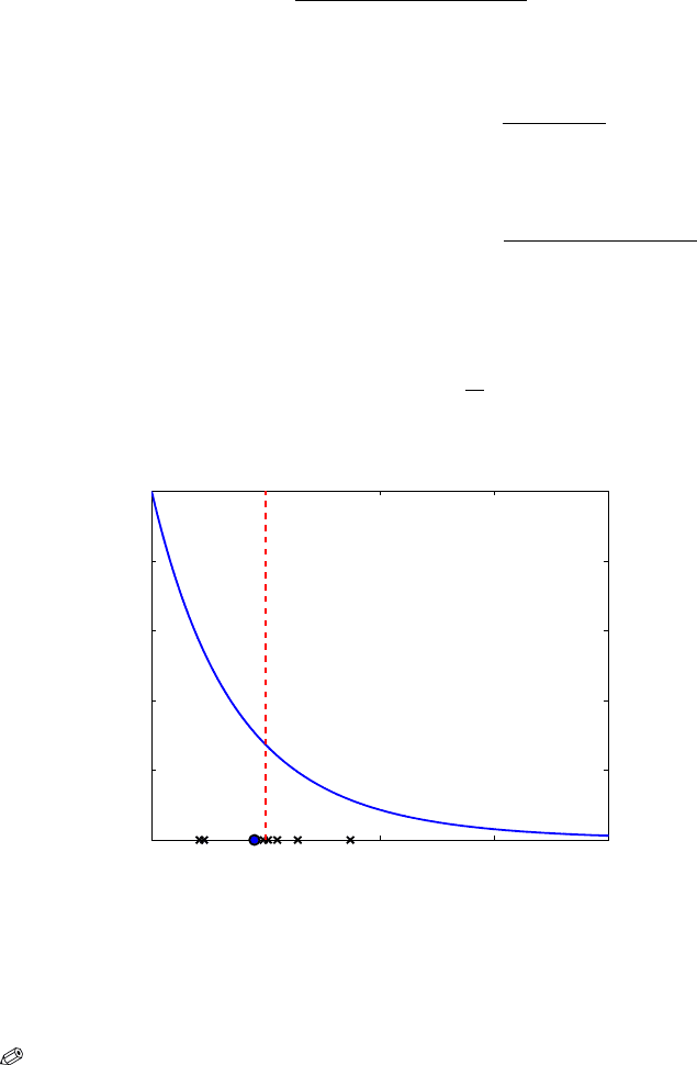
For example, if X

= 2.1, X

= 5.5, X

= 6.4, X

= 8.7, X

= 4.9, X

= 5.1,

and X

= 2.3 are the observations, and α = 2 and β = 1, then

= 9/2 and

=729/28 =26.0357. Figure 8.8 shows the posterior predictive distribution

(solid blue line), observations (crosses), and prediction for the new observation

(blue dot). The position of the mean of the data,

X = 5, is shown as a dotted

red line.

0 5 10 15 20

0.05

0.1

0.15

0.2

0.25

Fig. 8.8 Bayesian prediction (blue dot) based on the sample (black crosses) X = [2.1,

5.5, 6.4, 8.7, 4.9, 5.1, 2.3]

from the exponential distribution E (λ). The parameter

λ is given a gamma G a(2,1) distribution and the resulting posterior predictive distribution

is shown as a solid blue line. The position of the sample mean is plotted as a dotted red line.

8.10 Consensus Means* 305

Example 8.16. To ﬁnd the Bayesian prediction in WinBUGS, one simply sam-

ples a new observation from a likelihood that has updated parameters. In the

WinBUGS program below that implements Example 8.15, the observations

are read within the

for loop. However, if a new variable is simulated from the

same likelihood, this is done for the current version of the parameter

λ and the

mean of simulations approximates the posterior mean of the new observation.

model{

for (i in 1:7){

X[i] ~ dexp(lambda)

}

lambda ~ dgamma(2,1)

Xnew ~ dexp(lambda)

}

DATA

list(X = c(2.1, 5.5, 6.4, 8.7, 4.9, 5.1, 2.3))

INITS

list(lambda=1, Xnew=1)

The output is

mean sd MC error val2.5pc median val97.5pc start sample

Xnew 4.499 5.09 0.005284 0.1015 2.877 18.19 1001 100000

lambda 0.25 0.08323 8.343E-5 0.1142 0.2409 0.4378 1001 100000

Note that the posterior mean for Xnew is well approximated, 4.499 ≈ 4.5,

and that the standard deviation

sd = 5.09 is close to

26.0357 =5.1025.

8.10 Consensus Means*

Suppose that several labs are reporting measurements of the same quantity

and that a consensus mean should be calculated. This problem appears in

interlaboratory studies, as well as in multicenter clinical trials and various

meta-analyses. In this section we provide a Bayesian solution to this problem

and compare it with some classical proposals.

Let Y

i j

, i = 1,... , k; j = 1,. .., n

be measurements made at k laboratories,

where n

measurements come from lab i. Let n =

be the total sample

size.

We are interested in estimating the mean that would properly incorporate

information coming from all the labs, the so-called consensus mean. Why is

the solution not trivial and what is wrong with the average

Y = 1/n

i j

There is nothing wrong, under the proper conditions: (a) variabilities

within the labs must be equal and (b) there must be no variability between

the labs.

When (a) is relaxed, proper pooling of the lab sample means is done via a

Graybill–Deal estimator:

306 8 Bayesian Approach to Inference

, ω

When both conditions (a) and (b) are relaxed, there are many competing

classical estimators. For example, the Schiller–Eberhardt estimator is given

, ω

where s

is an estimator of the variance between the labs, s

(

max

−

min

)

The Mandel–Paule is the same as the Schiller–Eberhardt estimator but with

obtained iteratively.

The Bayesian approach is conceptually simple. Individual means as ran-

dom variables are generated from a single distribution. The mean of this dis-

tribution is the consensus mean. In somewhat convoluted wording, the con-

sensus mean is the mean of a hyperprior placed on the individual means.

Example 8.17. Selenium in Milk Powder. The data on selenium in non-

fat milk powder

selenium.dat are adapted from Witkovsky (2001). Four

independent measurement methods are applied. The Bayes estimator of the

consensus mean is 108.8.

In the WinBUGS program below, the individual means

theta[i] have a t-

prior with location

mu, precision tau, and 5 degrees of freedom. The choice of

t-prior, instead of the usual normal, is motivated by robustness considerations.

model{

for (i in 1:n)

{

sel[i] ~ dnorm( theta[lab[i]], prec[lab[i]])

}

for (i in 1:k)

{

theta[i] ~ dt(mu, tau,5) #individual means

prec[i] ~ dgamma(0.0001, 0.0001)

sigma2[i] <- 1/prec[i]

}

mu ~ dt(0,0.0001,5) #consensus mean

tau ~ dgamma(0.0001,0.0001)

si2 <-1/tau

}

DATA

list(lab=c(1,1,1,1,1,1,1,1, 2,2,2,2,2,2,2,2,2,2,2,2,

8.10 Consensus Means* 307

3,3,3,3,3,3,3,3,3,3,3,3,3,3, 4,4,4,4,4,4,4,4),

sel = c(

115.7, 113.5, 103.3, 119.1, 114.2, 107.3, 91.2, 104.4,

108.6, 109.1, 107.2, 111.5, 100.6, 106.3, 105.9, 109.7,

111.1, 107.9, 107.9, 107.9,

107.6, 107.26,109.7, 109.7, 108.5, 106.5, 110.2, 108.3,

110.5, 108.5, 108.8, 110.1, 109.4, 112.4,

118.7, 109.7, 114.7, 105.4, 113.9, 106.3, 104.8, 106.3),

k=4, n=42)

INITS

list( mu=1, tau=1, prec=c(1,1,1,1), theta=c(1,1,1,1) )

mean sd MC error val2.5pc median val97.5pc start sample

mu 108.8 0.6499 0.003674 107.6 108.9 110.0 5001 500000

si2 0.7252 9.456 0.02088 1.024E-4 0.01973 4.875 5001 500000

theta[1] 108.8 0.8593 0.003803 107.0 108.9 110.5 5001 500000

theta[2] 108.7 0.6184 0.004188 107.2 108.7 109.7 5001 500000

theta[3] 108.9 0.4046 0.00311 108.1 108.9 109.7 5001 500000

theta[4] 108.9 0.7505 0.003705 107.6 108.9 110.7 5001 500000

Next, we compare the Bayesian estimator with the classical Graybill–Deal

and Schiller–Eberhardt estimators, 108.8892 and 108.7703, respectively. The

Bayesian estimator falls between the two classical ones. A 95% credible set for

the consensus mean is [107.6, 110].

lab1=[115.7, 113.5, 103.3, 119.1, 114.2, 107.3, 91.2, 104.4];

lab2=[108.6, 109.1, 107.2, 111.5, 100.6, 106.3, 105.9, 109.7,...

111.1, 107.9, 107.9, 107.9];

lab3=[107.6, 107.26,109.7, 109.7, 108.5, 106.5, 110.2, 108.3,...

110.5, 108.5, 108.8, 110.1, 109.4, 112.4];

lab4=[118.7, 109.7, 114.7, 105.4, 113.9, 106.3, 104.8, 106.3];

m = [mean(lab1) mean(lab2) mean(lab3) mean(lab4)];

s = [std(lab1) std(lab2) std(lab3) std(lab4) ];

ni=[8 12 14 8]; k=length(m);

%Graybill-Deal Estimator

wei = ni./s.^2; %weights

gd = sum(m .

wei)/sum(wei) %108.8892

%Schiller-Eberhardt Estimator

z = sort(m);

sb2 = (z(k)-z(1))^2/12;

wei = 1./(s.^2./ni + sb2);%weights

se = sum(m .

wei)/sum(wei) %108.7703

Borrowing Strength and Vague Priors. As popularly stated, this model

allows for borrowing strength in the estimation of both the means

and the