Vidakovic B. Statistics for Bioengineering Sciences: With Matlab and WinBugs Support

Подождите немного. Документ загружается.

11.7 Power Analysis in ANOVA 439

0 500 1000 1500 2000 2500

0.2

0.4

0.6

0.8

1.2

1.4

1.6

1.8

Sums of Squares

SSA

SSB

SSE

SST

Fig. 11.6 The budget of sums of squares for the mouse-diet study.

hypothesis H

: α

=α

=···=α

=0. It quantiﬁes the extent of deviation from

and usually is a function of the ratio

Under H

, for a balanced design, the test statistic F has an F-distribution

with k

−1 and N −k = k(n −1) degrees of freedom, where k is the number of

treatments and n the number of subjects at each level.

However, if H

is not true, the test statistic has a noncentral F-distribution

with k

−1 and k(n −1) degrees of freedom and a noncentrality parameter λ =

An alternative way to set the precision is via Cohen’s effect size, which

for ANOVA takes the form f

1/k

. Note that Cohen’s effect size and

noncentrality parameter are connected via

λ = N f

= nk f

Since determining the sample size is a prospective task, information about

and α

may not be available. In the context of ANOVA Cohen (1988) recom-

mends effect sizes of f

= 0.1

as small, f

= 0.25

as medium, and f

= 0.4

as large.

The power in ANOVA is, by deﬁnition,

−β =P(F

(k −1, N −k,λ) >F

−1

(1 −α, k −1, N −k)), (11.5)

where F

(k −1, N − k,λ) is a random variable with a noncentral F-

distribution with k

−1 and N −k degrees of freedom and noncentrality

440 11 ANOVA and Elements of Experimental Design

parameter λ. The quantity F

−1

(1 −α, k −1, N −k) is the 1 −α percentile

(a cut point for which the upper tail has a probability

α) of a standard

F-distribution with k

−1 and N −k degrees of freedom.

The interplay among the power, sample size, and effect size is illustrated

by the following example.

Example 11.8. Suppose k

=4 treatment means are to be compared at a signif-

icance level of

α =0.05. The experimenter is to decide how many replicates n

to run at each level, so that the null hypothesis is rejected with a probability

of at least 0.9 if f

=0.0625 or if

is equal to σ

/4.

For n

=60, i.e., N =240, the power is calculated in a one-line command:

1-ncfcdf(finv(1-0.05, 4-1, 4

(60-1)), 4-1, 4

(60-1), 15) %0.9122

Here we used λ = nk f

=60 ×4 ×0.0625 =15.

One can now try different values of n (group sample sizes) to achieve

the desired power; this change affects only two arguments in Eq. (11.5):

k(n

−1) and λ = nk f

. Alternatively, one can use MATLAB’s built in function

fzero(fun,x0) which tries to ﬁnd a zero of fun near some initial value x0.

k=4; alpha = 0.05; f2 = 0.0625;

f = @(n) 1-ncfcdf( finv(1-alpha, k-1,k

n-k),k-1,k

n-k, n

f2 ) - 0.90;

ssize = fzero(f, 100) %57.6731

%Sample size of n=58 (per treatment) ensures the power of 90% for

%the effect size f^2=0.0625.

Thus, sample size of n = 58 will ensure the power of 90% for the speciﬁed

effect size. The function

fzero is quite robust with respect to speciﬁcation of

the initial value; in this case the initial value was n

=100.

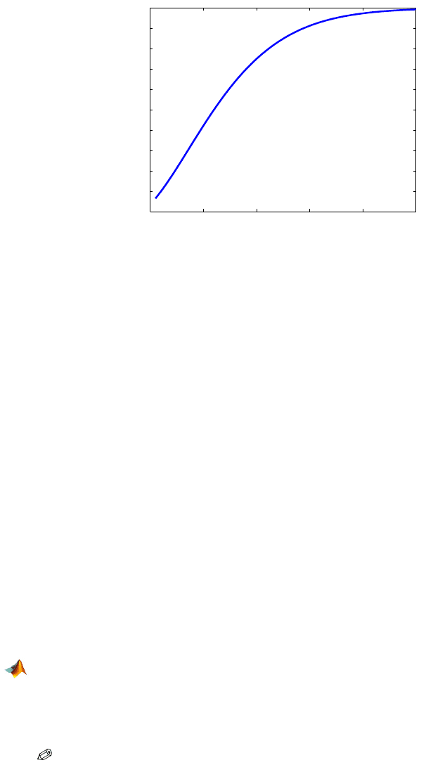
If we wanted to plot the power for different sample sizes (Fig. 11.7), the

following simple MATLAB script would do it. The inputs are the k number

of treatments and the signiﬁcance level

α. The speciﬁc alternative H

is such

that

=σ

/4, so that λ = n/4.

k=4; %number of treatments

alpha = 0.05; %significance level

y=[]; %set values of power for n

for n=2:100

y =[y 1-ncfcdf(finv(1-alpha, k-1, k

(n-1)), ...

k-1, k

(n-1), n/4)];

end

plot(2:100, y,’b-’,’linewidth’,3)

xlabel(’Group sample size n’); ylabel(’Power’)

In the above analysis, the total sample size is N = k ×n =240.

11.7 Power Analysis in ANOVA 441

0 20 40 60 80 100

0.1

0.2

0.3

0.4

0.5

0.6

0.7

0.8

0.9

Group sample size n

Power

Fig. 11.7 Power for n ≤100 (size per group) in a ﬁxed-effect ANOVA with k =4 treatments

and

α =0.05. The alternative H

is deﬁned as

=σ

/4 so that the parameter of noncen-

trality

λ is equal to n/4.

Sample Size for Multifactor ANOVA. A power analysis for multifactor

ANOVA is usually done by selecting the most important factor and evaluating

the power for that factor. Operationally, this is the same as the previously

discussed power analysis for one-way ANOVA, but with modiﬁed error degrees

of freedom to account for the presence of other factors.

Example 11.9. Assume two-factor, ﬁxed-effect ANOVA. The test for factor A at

=4 levels is to be evaluated for its power. Factor B is present and has b =3

levels. Assume a balanced design with 4

×3 cells, with n = 20 subjects in each

cell. The total number of subjects in the experiment is N

=3 ×4 ×20 =240.

For

α = 0.05, a medium effect size f

= 0.0625, and λ = N f

= 20 ×4 ×3 ×

0.0625 =15, the power is 0.9121.

1-ncfcdf(finv(1-0.05, 4-1, 4

(20-1)), 4-1, 4

(20-1), 15) %0.9121

Alternatively, if the cell sample size n is required for a speciﬁed power we

can use function

fzero.

a=4; b=3; alpha = 0.05; f2=0.0625;

f = @(n) 1-ncfcdf( finv(1-alpha, a-1,a

(n-1)), ...

a-1, a

(n-1), a

f2) - 0.90;

ssize = fzero(f, 100) %19.2363

%sample size of 20 (by rounding 19.2363 up) ensures 90% power

%given the effect size and alpha

442 11 ANOVA and Elements of Experimental Design

Sample Size for Repeated Measures Design. In a repeated measures

design, each of the k treatments is applied to every subject. Thus, the total

sample size is equal to a treatment sample size, N

= n. Suppose that ρ is the

correlation between scores for any two levels of the factor and it is assumed

constant. Then the power is calculated by Eq. (11.5), where the noncentrality

parameter is modiﬁed as

λ =

(1 −ρ)σ

nk f

1 −ρ

Example 11.10. Suppose that n

=25 subjects go through k =3 treatments and

that a correlation between the treatments is

ρ = 0.6. This correlation comes

from the experimental design; the measures are repeated on the same sub-

jects. Then for the medium effect size (f

= 0.25 or f

= 0.0625) the achieved

power is 0.8526.

n=25; k=3; alpha=0.05; rho=0.6;

f = 0.25; %medium effect size f^2=0.0625

lambda = n

f^2/(1-rho) %11.7188

power = 1-ncfcdf( finv(1-alpha, k-1, (n-1)

(k-1)),...

k-1, (n-1)

(k-1), lambda) %0.8526

If the power is speciﬁed at 85% level, then the number of subjects is ob-

tained as

k=3; alpha=0.05; rho=0.6; f=0.25;

pf = @(n) 1-ncfcdf( finv(1-alpha, k-1, (n-1)

(k-1)),...

k-1, (n-1)

(k-1), n

f^2/(1-rho) ) - 0.85;

ssize = fzero(pf, 100) %24.8342 (n=25 after rounding)

Often the sphericity condition is not met. This happens in longitudinal

studies (repeated measures taken over time) where the correlation between

measurements on days 1 and 2 may differ from the correlation between days

1 and 4, for example. In such a case, average correlation

ρ is elicited and used;

however, all degrees of freedom in central and noncentral F, as well as

λ, are

multiplied by sphericity parameter

².

Example 11.11. Suppose, as in Example 11.10, that n

=25 subjects go through

= 3 treatments, and that an average correlation between the treatments is

ρ = 0.6. If the sphericity is violated and parameter ² is estimated as ² = 0.7,

the power of 85.26% from Example 11.10 drops to 74.64%.

n=25; k=3; alpha=0.05; barrho=0.6; eps=0.7;

f = 0.25;

11.8 Functional ANOVA* 443

lambda = n

f^2/(1-barrho) %11.7188

power = 1-ncfcdf( finv(1-alpha, eps

(k-1), eps

(n-1)

(k-1)),...

eps

(k-1), eps

(n-1)

(k-1), eps

lambda) %0.7464

If the power is to remain at 85% level, then the number of subjects should

increase from 25 to 32.

k=3; alpha=0.05; barrho=0.6; eps=0.7; f = 0.25;

pf = @(n) 1-ncfcdf( finv(1-alpha, eps

(k-1), eps

(n-1)

(k-1)),...

eps

(k-1), eps

(n-1)

(k-1), eps

f^2/(1-barrho) ) - 0.85;

ssize = fzero(pf, 100) %31.8147

11.8 Functional ANOVA*

Functional linear models have become popular recently since many responses

are functional in nature. For example, in an experiment in neuroscience, ob-

servations could be functional responses, and rather than applying the experi-

mental design on some summary of these functions, one could use the densely

sampled functions as data.

We provide a deﬁnition for the one-way case, which is a “functionalized”

version of standard one-way ANOVA.

Suppose that for any ﬁxed t

∈ T ⊂ R, the observations y are modeled by a

ﬁxed-effect ANOVA model:

i j

(t) =µ(t) +α

(t) +²

i j

(t), i =1,..., k, j =1,... , n

;

i=1

= N, (11.6)

where

i j

(t) are independent N (0,σ

) errors. When i and j are ﬁxed, we as-

sume that functions

µ(t) and α

(t) are square-integrable functions. To ensure

the identiﬁability of treatment functions

, one typically imposes

(

∀t)

(t) =0. (11.7)

In real life the measurements y are often taken at equidistant times t

The standard least square estimators for

µ(t) and α

(t)

µ(t) = y(t) =

i, j

i j

(t), (11.8)

(t) = y

(t) − y(t), (11.9)

where

(t) =

i j

(t), are obtained by minimizing the discrete version of

LMSSE [for example, Ramsay and Silverman (1997) p. 141],

LMSSE

i, j

i j

(t) −(µ(t)+α

(t))]

, (11.10)

444 11 ANOVA and Elements of Experimental Design

subject to the constraint (∀t)

(t) =0.

The fundamental ANOVA identity becomes a functional identity,

SST(t)

=SSTr(t) +SSE(t), (11.11)

with SST(t)

i,l

(t) − y(t)]

, SSTr(t) =

(t) − y(t)]

, and SSE(t) =

i,l

(t) − y

(t)]

For each t, the function

F(t)

SSTr(t)/(k −1)

SSE(t)/(N −k)

(11.12)

is distributed as noncentral F

k−1,N−k

(t)

. Estimation of µ(t) and α

(t)

is straightforward, and estimators are given in Eqs. (11.8).

The testing of hypotheses involving functional components of the stan-

dard ANOVA method is hindered by dependence and dimensionality problems.

Testing requires dimension reduction and this material is beyond the scope of

this book. The interested reader can consult Ramsay and Silverman (1997)

and Fan and Lin (1998).

Example 11.12. FANOVA in Tumor Physiology. Experiments carried out

in vitro with tumor cell lines have demonstrated that tumor cells respond to

radiation and anticancer drugs differently, depending on the environment. In

particular, available oxygen is important. Efforts to increase the level of oxy-

gen within tumor cells have included laboratory rats with implanted tumors

breathing pure oxygen. Unfortunately, animals breathing pure oxygen may

experience large drops in blood pressure, enough to make this intervention

too risky for clinical use.

Mark Dewhirst, Department of Radiation Oncology at Duke University,

sought to evaluate carbogen (95% pure oxygen and 5% carbon dioxide) as a

breathing mixture that might improve tumor oxygenation without causing

a drop in blood pressure. The protocol called for making measurements on

each animal over 20 minutes of breathing room air, followed by 40 minutes

of carbogen breathing. The experimenters took serial measurements of oxy-

gen partial pressure (PO

), tumor blood ﬂow (LDF), mean arterial pressure

(MAP), and heart rate. Microelectrodes, inserted into the tumors (one per ani-

mal), measured PO

at a particular location within the tumor throughout the

study period. Two laser Doppler probes, inserted into each tumor, provided

measurements of blood ﬂow. An arterial line into the right femoral artery al-

lowed measurement of MAP. Each animal wore a face mask for administration

of breathing gases (room air or carbogen). [See Lanzen et al. (1998) for more

information about these experiments.]

Nine rats had tumors transplanted within the quadriceps muscle (which

we will denote by TM). For comparison, the studies also included eight rats

with tumors transplanted subcutaneously (TS) and six rats without tumors

11.8 Functional ANOVA* 445

(N) in which measurements were made in the quadriceps muscle. The data

are provided in

oxigen.dat.

20 40 60

t (min)

Treatment 1

20 40 60

t (min)

Treatment 1

20 40 60

t (min)

Treatment 1

20 40 60

t (min)

Treatment 1

20 40 60

t (min)

Treatment 1

20 40 60

t (min)

Treatment 1

20 40 60

t (min)

Treatment 2

20 40 60

t (min)

Treatment 2

20 40 60

t (min)

Treatment 2

20 40 60

t (min)

Treatment 2

20 40 60

t (min)

Treatment 2

20 40 60

t (min)

Treatment 3

20 40 60

t (min)

Treatment 3

20 40 60

t (min)

Treatment 3

20 40 60

t (min)

Treatment 3

20 40 60

t (min)

Treatment 3

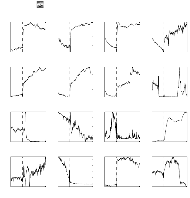
Fig. 11.8 PO

measurements. Notice that despite a variety of functional responses and a

lack of a simple parametric model, at time t

∗

=20

the pattern generally changes.

Figure 11.8 show some of the data (PO

). The plots show several features,

including an obvious rise in PO

at the 20-minute mark among some of the

animals. No physiologic model exists that would characterize the shapes of

these proﬁles mathematically. The primary study question concerned evaluat-

ing the effect of carbogen breathing on PO

. The analysis was complicated by

the knowledge that there may be acute changes in PO

after carbogen breath-

ing starts. The primary question of interest is whether the tumor tissue be-

haves differently than normal muscle tissue or whether a tumor implanted

subcutaneously responds to carbogen breathing differently than tumor tissue

implanted in muscle tissue in the presence of acute jumps in PO

446 11 ANOVA and Elements of Experimental Design

The analyses concern inference on changes in some physiologic measure-

ments after an intervention. The problem for the data analysis is how best to

deﬁne “change” to allow for the inference desired by the investigators.

From a statistical modeling point of view, the main issues concern building

a ﬂexible model for the multivariate time series y

i j

of responses and providing

for formal inference on the occurrence of change at time t

∗

and the “equality”

of the PO

proﬁles. From the ﬁgures it is clear that the main challenge arises

from the highly irregular behavior of responses. Neither physiologic consid-

erations nor any exploratory data analysis motivates any parsimonious para-

metric form. Different individuals seem to exhibit widely varying response

patterns. Still, it is clear from inspection of the data that for some response

series a deﬁnite change takes place at time t

∗

20 40 60

t (min)

µ(t)

20 40 60

t (min)

(t)

20 40 60

−20

−15

−10

−5

t (min)

(t)

20 40 60

t (min)

(t)

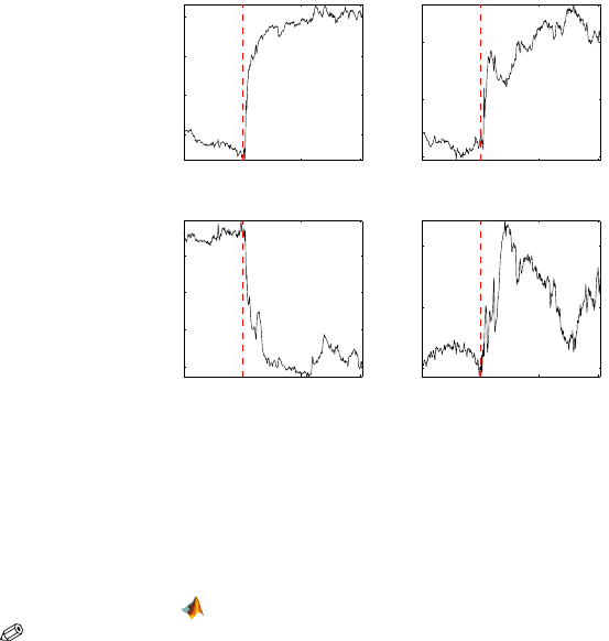
Fig. 11.9 Functional ANOVA estimators.

Figure 11.9 shows the estimators of components in functional ANOVA. One

can imagine from the ﬁgure that adding

µ(t) and α

(t) will lead to a relatively

horizontal expected proﬁle for group i, each ﬁtted curve canceling the other to

some extent. Files

micePO2.m and fanova.m support this example.

11.9 Analysis of Means (ANOM)*

Some statistical applications, notably in the area of quality improvement, in-

volve a comparison of treatment means to determine which are signiﬁcantly

11.9 Analysis of Means (ANOM)* 447

different from their overall average. For example, a biomedical engineer might

run an experiment to investigate which of six concentrations of an agent pro-

duces different output, in the sense that the average measurement for each

concentration differs from the overall average.

Questions of this type are answered by the analysis of means (ANOM),

which is a method for making multiple comparisons that is sometimes referred

to as a “multiple comparison with the weighted mean”. The ANOM answers

different question than the ANOVA; however, it is related to ANOVA via mul-

tiple tests involving contrasts (Halperin et al., 1955; Ott, 1967)

The ANOM procedure consists of multiple testing of k hypotheses H

: α

0, i =1, ..., k versus the two sided alternative. Since the testing is simultane-

ous, the Bonferroni adjustment to the type I error is used. Here

are, as in

ANOVA, k population treatment effects

−µ, i =1,..., k which are estimated

= y

− y,

in the usual ANOVA notation. Population effect

can be represented via the

treatment means as

= µ

−µ =µ

−

+···+µ

= −

−···−

i−1

1 −

−···−

Since the constants c

=−1/k, ... , c

=1 −1/k, . .., c

=−1/k sum up to 0,

an empirical contrast,

= y

−

+···+ y

= −

−···−

i−1

1 −

−···−

with standard deviation (as in p. 417),

= s

j=1

= s

1 −

j6=i

Here n

are treatment sample sizes, N =

is the total sample size, and

MSE.

All effects

falling outside the interval

[

−s

×t

N−k,1−α/(2k)

, s

×t

N−k,1−α/(2k)

or equivalently, all treatment means

falling outside of the interval

448 11 ANOVA and Elements of Experimental Design

[y −s

×t

N−k,1−α/(2k)

, y +s

×t

N−k,1−α/(2k)

correspond to rejection of H

: α

= µ

−µ = 0. The Bonferroni correction 1 −

α/(2k) in the t-quantile t

N−k,1−α/(2k)

controls the signiﬁcance of the procedure

at level

α (p. 342).

Example 11.13. We revisit Example 11.1 (Coagulation Times) and perform

an ANOM analysis. In this example

= 61, y

= 66, y

= 68, and y

= 61.

The grand mean is

y = 64. Standard deviations for

α are s

= 0.9736, s

0.8453, s

= 0.8453, and s

= 0.7733, while the t-quantile corresponding to

α = 0.05 is t

1−0.05/8,20

= 2.7444. This leads to ANOM bounds, [61.328,66.672],

[61.680,66.320], [61.680,66.320], and [61.878,66.122].

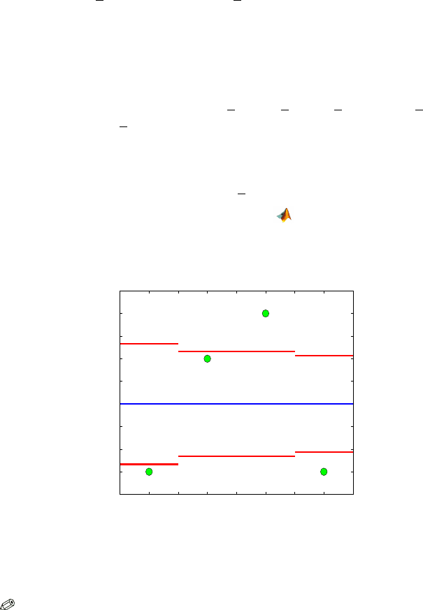
Only the second treatment mean

= 66 falls in its ANOM interval

[61.680, 66.320], see Fig. 11.10 (generated by

anomct.m). Consequently, the

second population mean

is not signiﬁcantly different from the grand mean

µ.

0.5 1 1.5 2 2.5 3 3.5 4 4.5

Fig. 11.10 ANOM analysis in example Coagulation Times. Blue line is the overall mean,

red lines are the ANOM interval bounds, while green dots are the treatment means. Note

that only the second treatment mean falls in its interval.

11.10 The Capability of a Measurement System (Gauge

R&R ANOVA)*

The gauge R&R methodology is concerned with the capability of measur-

ing systems. Over time gauge R&R methods have evolved, and now two ap-