Wai-Fah Chen.The Civil Engineering Handbook

55-36 The Civil Engineering Handbook, Second Edition

or

(55.167)

with C = GM. Rather than solving for three second-order differential equations (DEs), we make a

transformation to six ﬁrst-order DEs. Introduce three new variables U, V, W:

(55.168)

Equations (55.162) through (55.165) yield the following six DEs:

(55.169)

Integration of Eq. (55.169) results in six constants of integration. One is free to choose at an epoch t

0

six variables, {X

0

, Y

0

,

Z

0

,

U

0

,

V

0

,

W

0

} or {X

0

, Y

0

,

Z

0

,

·

X

0

,

·

Y

0

,

·

Z

0

}. These six starting values determine uniquely

the orbit of m around M. In other words, if we know the position {X

0

, Y

0

,

Z

0

} and its velocity {

·

X

0

,

·

Y

0

,

·

Z

0

}

at an epoch t

0

, then we are able to determine the position and velocity of m at any other epoch t by

numerical integration of Eq. (55.169).

Analytical Solution of Three Second-Order Differential Equations

The differential equations of an earth-orbiting satellite can also be solved analytically. Without derivation,

the solution is presented in computational steps in terms of transformation formulas.

In history the solution to the motion of planets around the sun was found before its explanation.

Through the analysis of his own observations and those made by Tycho Brahe, Johannes Kepler discovered

certain regularities in the motions of planets around the sun and formulated the following three laws:

1. Formulated 1609: The orbit of each planet around the sun is an ellipse. The sun is in one of the

two focal points.

2. Formulated 1609: The sun–planet line sweeps out equal areas in equal time periods.

3. Formulated 1611: The ratio between the square of a planet’s orbital period and the third power

of its average distance from the sun is constant.

Kepler’s third law leads to the famous equation

(55.170)

˙˙

/

XCXX Y Z

YCYX Y Z

ZCZX Y Z

=++

()

È

Î

Í

˘

˚

˙

=++

()

È

Î

Í

˘

˚

˙

=++

()

È

Î

Í

˘

˚

˙

222

32

222

32

222

32

UX

dX

dt

VY

dY

dt

WZ

dZ

dt

== == ==

˙

;

˙

;

˙

UX

VY

WZ

UCXX Y Z

VCYX Y Z

WCZX Y Z

=

=++

()

È

Î

Í

˘

˚

˙

=++

()

È

Î

Í

˘

˚

˙

=++

()

È

Î

Í

˘

˚

˙

/

222

32

222

32

222

32

na GM

23

=

Geodesy 55-37

in which n is the average angular rate and a the semimajor axis of the orbital ellipse.

In 1665–1666 Newton formulated his more fundamental laws of nature (which were only published

after 1687) and showed that Kepler’s laws follow from them.

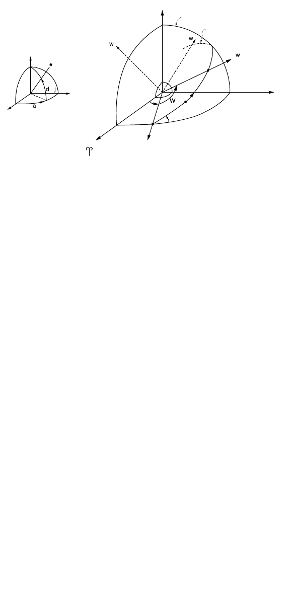
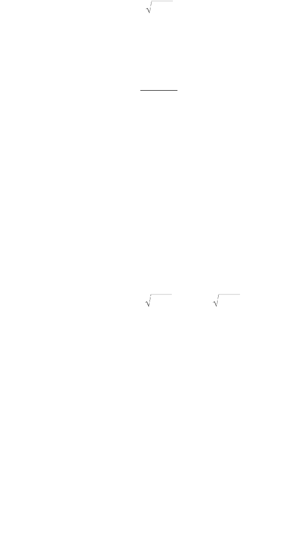
Orientation of the Orbital Ellipse

In a (quasi-)inertial frame the ellipse of an earth-orbiting satellite has to be positioned: the focal point

will coincide with the center of mass of the earth. Instead of picturing the ellipse itself we project the

ellipse on a celestial sphere centered at the CoM. On the celestial sphere we also project the earth’s equator

(see Fig. 55.18).

The orientation of the orbit ellipse requires three orientation angles with respect to the inertial frame

XYZ: two for the orientation of the plane of the orbit (W and I) and one for the orientation of the ellipse

in the orbital plane in terms of the point of closest approach, the perigee (w).

W represents the right ascension (a) of the ascending node. The ascending node is the (projected)

point where the satellite rises above the equator plane. I represents the inclination of the orbital plane

with respect to the equator plane. w represents the argument of perigee: the angle from the ascending

node (in the plane of the orbit) to the perigee (for planets, the perihelion), which is that point where

the satellite (planet) approaches closest to the earth (sun) or, more precisely, the CoM of the earth (sun).

We deﬁne now another reference frame X

w

, of which the X

w

Y

w

plane coincides with the orbit plane.

The X

w

axis points to the perigee, and the origin coincides with the earth’s CoM (∫ focal point ellipse ∫

origin of X frame). The relationship between the inertial frames X

I

and X

w

is

(55.171)

in which

(55.172)

and

(55.173)

FIGURE 55.18 Celestial sphere with projected orbit ellipse and equator.

Z

Y

X

=

Celestial sphere

Projected orbital ellipse

Perigee

X

Z

Y

Z

Y

i

Ascending node

X

Ω

X

II

= RX

??

RR R R

?3 1 3I

I=-

()

-

()

-

()

Ww

X

w

=

Ê

Ë

Á

ˆ

¯

˜

X

Y

Z 0

55-38 The Civil Engineering Handbook, Second Edition

Reference Frame in the Plane of the Orbit

Now that we know the orientation of the orbital ellipse we have to deﬁne the size and shape of the ellipse

and the position of the satellite along the ellipse at a certain epoch t

0

.

Similarly to the earth’s ellipsoid, discussed in Section 55.2, we deﬁne the ellipse by a semimajor axis

a and eccentricity e. In orbital mechanics it is unusual to describe the shape of the orbital ellipse by its

ﬂattening.

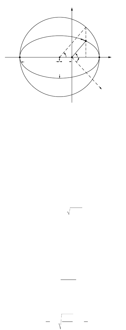
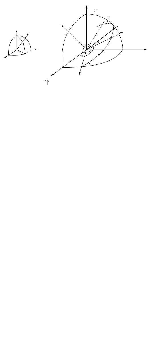
The position of the satellite in the orbital X

w

Y

w

plane is depicted in Fig. 55.19. In the ﬁgure the auxiliary

circle enclosing the orbital ellipse reveals the following relationships:

(55.174)

(55.175)

in which

(55.176)

In Fig. 55.19 and the Eqs. (55.174) through (55.176), a is the the semimajor axis of the orbital ellipse,

b is the semiminor axis of the orbital ellipse, e is the eccentricity of the orbital ellipse, with

(55.177)

n is the the true anomaly, sometimes denoted by an f, and E is the eccentric anomaly.

The relation between the true and the eccentric anomalies can be derived to be

(55.178)

Substitution of Eqs. (55.174) through (55.176) into (55.171) gives

FIGURE 55.19 The position of the satellite S in the orbital plane.

Apogee

a

b

ae

E

a

S

Perigee

X

w

Y

w

r

w

Ascending node

u

Xr a Ee

ww

n==-

()

cos cos

Yr a e E

ww

n==-sin sin1

2

ra eE

w

=-

()

1 cos

e

ab

a

2

22

2

=

-

tan tan

E

e

e2

1

12

Ê

Ë

Á

ˆ

¯

˜

=

-

+

Ê

Ë

Á

ˆ

¯

˜

n

Geodesy 55-39

(55.179)

In Eq. (55.179) the Cartesian coordinates are expressed in the six so-called Keplerian elements: a, e,

I, W, w, and E. Paraphrasing an earlier remark: if we know the position of the satellite at an epoch t

0

through {a, e, I, W, w, and E

0

}, we are capable of computing the position of the satellite at an arbitrary

epoch t through the Eq. (55.179) if we know the relationship in time between E and E

0

. In other words,

how does the angle E increase with time?

We deﬁne an auxiliary variable (angle) M, which increases linearly in time with the mean motion

n (= (GM/a

3

)

1/2

) according to Kepler’s third law. The angle M, the mean anomaly, may be expressed as

function of time by

(55.180)

Through Kepler’s equation

(55.181)

the (time) relationship between M and E is given. Kepler’s equation is the direct result of the enforcement

of Kepler’s second law (equal area law).

Combining Eqs. (55.180) and (55.181) gives an equation that expresses the relationship between a

given eccentric anomaly E

0

(or M

0

or n

0

) at an epoch t

0

and the eccentric anomaly E at an arbitrary epoch t:

(55.182)

Transformation from Keplerian to Cartesian Orbital Elements

So far, the position vector {X, Y, Z} of the satellite has been expressed in terms of the Keplerian elements.

The transformation is complete when we express the velocity vector {

·

X

0

,

·

Y

0

,

·

Z

0

} in terms of those Keple-

rian elements. Differentiating Eq. (55.171) with respect to time we get

(55.183)

Since we consider the two-body problem with m

1

= M ? m = m

2

, the orientation of the orbital ellipse

is time independent in the inertial frame. This means that the orientation angles I, W, w are time

independent as well:

(55.184)

Equation (55.183) simpliﬁes to

(55.185)

Differentiating Eqs. (55.174) through (55.176) with respect to time we have

(55.186)

XRRR

I313

=

Ê

Ë

Á

ˆ

¯

˜

=-

()

-

()

-

()

-

()

-

Ê

Ë

Á

ˆ

¯

˜

X

Y

Z

I

aEe

aeEWw

cos

sin1

0

2

MM ntt=+-

()

00

MEe E=-sin

EE e E E ntt-= -

()

+-

()

000

sin sin

˙˙˙

XRXRX

I? ? ? ?II

=+

˙

[]R

Iw

= 0

˙˙

XRX

I

=

I??

˙

sin

X

w

=-aE E

55-40 The Civil Engineering Handbook, Second Edition

(55.187)

(55.188)

The remaining variable

·

E is obtained through differentiation of Eq. (55.181):

(55.189)

Now all transformation formulas express the Cartesian orbital elements (state vector elements) in

terms of the six Keplerian elements:

(55.190)

or

(55.191)

(55.192)

Transformation from Cartesian to Keplerian Orbital Elements

To compute the inertial position of a satellite in a central force ﬁeld, it is simpler to perform a time

update in the Keplerian elements than in the Cartesian elements. The time update takes place in Eqs.

(55.180) through (55.182).

Schematically the following procedure is to be followed:

The conversion from Keplerian elements to state vector elements has been treated in the previous

subsection. In this section the somewhat more complicated conversion from position and velocity vector

to Keplerian representation will be described. Basically we “invert” Eq. (55.192) by solving for the six

elements {a, e, I, W, w, E

0

} in terms of the six state vector elements.

˙

cos

Y

w

=- -aE e E1

2

˙

sinraEe E

w

=

˙

cos

E

n

eE

=

-1

XX R X X

II I

◊

[]

= ◊

[]

˙˙

ww w

XX

II

X

Y

Z

X

Y

Z

◊

[]

=

◊

È

Î

Í

˘

˚

˙

=

˙

=-

()

-

()

-

()

-

()

◊

- ◊

◊

È

Î

Í

-

˘

˚

˙

RRR

313

W I

aEe

aeE

aE E

aE e Ew

cos

sin

˙

sin

˙

cos1

0

1

0

22

tXYZX

taeI

tXYZX

YZ

E

YZ

0

00

11

1

:,,,

˙

:,,,

˙

,

˙

,

˙

,,

,

˙

,

˙

{}

Ø

{}

Ø

{}

Ø

{}

Conversion to Keplerian elements, this subsection

Conversion to Keplerian, Eq. (55.182)

Conversion to Cartesian elements, previous subsection

W

w

Geodesy 55-41

First, we introduce another reference frame X

u

:

X

I

, Y

I

, Z

I

: inertial reference frame (X

I

axis Æ vernal equinox)

X

w

, Y

w

, Z

w

: orbital reference frame (X

w

axis Æ perigee)

X

u

, Y

u

, Z

u

: orbital reference frame (X

u

axis Æ satellite)

The X

u

frame is deﬁned similarly to the X

w

frame, except that the X

u

axis continuously points to the

satellites (see Fig. 55.20). Thus,

(55.193)

The angle in the orbital plane enclosed by the X

u

axis and the direction to the ascending node is called

u, the argument of latitude, with

(55.194)

As in the discussion of the orientation of the orbit ellipse, the following relationships hold:

(55.195)

(55.196)

(55.197)

Figure 55.20 reveals that

(55.198)

(55.199)

(55.200)

FIGURE 55.20 The orbital reference frame X

u

.

Z

X

Y

a

d=j

Z

S

Y

X

u

Z

w

X

u

X

w

Y

w

Ω

i

w

Projected orbital ellipse

Celestial sphere

Perigee

Ascending node

X

Y

Z

X

0

u

=

Ê

Ë

Á

ˆ

¯

˜

=

Ê

Ë

Á

ˆ

¯

˜

uv=+w

XRX

ww

=

II

XRX

uuII

=

XRXRRX

uu uII

==

?? ??

RRRR

w

II

I=

() () ()

33

W

RRRR

uI I

uI=

() () ( )

33

W

=+

()

() ( )

RRR

33

vI

I

wW

55-42 The Civil Engineering Handbook, Second Edition

(55.201)

(55.202)

We deﬁne a vector h perpendicular to the orbital plane according to

(55.203)

in which w is the unit vector along h. Consequently,

(55.204)

h represents the angular momentum vector (vector product of position vector and velocity vector). The

Keplerian elements W and I follow directly from Eqs. (55.203) and (55.204):

(55.205)

(55.206)

From

(55.207)

it follows that

(55.208)

(55.209)

and

(55.210)

Before determining the third Keplerian element deﬁning the orientation of the orbit (w) from the

argument of latitude (u), we deﬁne the following quantities:

•Length r of the radius vector X:

(55.211)

=

() ( ) () ( )

RR RR

33 3

vI

I

wW

=

()

=RR RR

3

v

IuIwww

hXXhwh

I

∫ ¥= = -

Ê

Ë

Á

ˆ

¯

˜

˙

sin

cos

W

I

h =

Ê

Ë

Á

ˆ

¯

˜

=

-

Ê

Ë

Á

ˆ

¯

˜

h

YZ ZY

ZX XZ

XY YX

1

2

3

˙

˙˙

tan W=

-

h

1

2

tan I

hh

h

=

+

1

2

3

RXRRX

3I3I

-

()

=

() ( )

uI

u

W

XuX Y

u

cos cos sin=+WW

XuXI YI ZI

u

sin cos sin cos cos sin=- + +WW

tan

– cos sin cos cos sin

cos sin

u

XI YI ZI

XY

=

++

+

WW

rXYZ∫ =++

()

X

222

12

Geodesy 55-43

•Length

·

r of the radial component of the velocity vector:

(55.212)

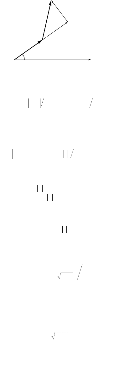
The Vis-Viva equation gives the relationship between the length (magnitude) V of the velocity vector

·

X and the length r of the position vector X through the radial component (

·

r) and the tangential com-

ponent (r

·

v) (see Fig. 55.21):

(55.213)

From Eq. (55.213) it follows that

(55.214)

In a similar manner one arrives at

(55.215)

From Eqs. (55.188), (55.189), (55.176), and (55.170) the eccentric anomaly E may be computed:

(55.216)

The mean anomaly M is given by

(55.217)

The true anomaly v follows from Eqs. (55.174) and (55.175):

(55.218)

after which, ﬁnally, the last Keplerian element, w, is determined through Eq. (55.194):

(55.219)

FIGURE 55.21 Illustration of the Vis-Viva equation.

X

•

(V)

(ru

•

)

(r

•

)

u

CoM

X

Perigee

˙

˙˙

˙

rrXXYYZZr∫◊ =++XX

VrrvrrGM

ra

2

222

2

21

∫ =+ =+ = -

Ê

Ë

Á

ˆ

¯

˜

˙

(

˙

)

˙

Xh

a

GM

GM V

rGM

GM rV

=

-

=

-

X

X22

22

1

2

-=e

aGM

h

tan

sin

cos

˙

E

rr

e GMa

ar

ae

==

Ê

Ë

Á

ˆ

¯

˜

-

Ê

Ë

Á

ˆ

¯

˜

MEe E=-sin

tan

sin

cos

v

eE

Ee

=

-

1

2

w= -uv

55-44 The Civil Engineering Handbook, Second Edition

Orbit of a Satellite in a Noncentral Force Field

The equations of motion for a real satellite are more difﬁcult than reﬂected by Eq. (55.165). First of all,

we do not deal with a central force ﬁeld: the earth is not a sphere, and it does not have a radial symmetric

density. Secondly, we deal with other forces, chieﬂy the gravity of the moon and the sun, atmospheric

drag, and solar radiation pressure. Equation (55.165) gets a more general meaning if we suppose that

the potential function is generated by the sum of the forces acting on the satellite:

(55.220)

with the central part of the earth’s gravitational potential

(55.221)

and the noncentral and time-dependent part of the earth’s gravitational ﬁeld

(55.222)

and so forth.

The superscript t has been added to various potentials to reﬂect their time variance with respect to

the inertial frame.

The equations of motion to be solved are

(55.223)

For the earth’s gravitational ﬁeld we have (in an earth-ﬁxed frame)

(55.224)

With Eq. (55.224) one is able to compute the potential at each point {l, f, r} necessary for the

integration of the satellite’s orbit. The coefﬁcients C

lm

and S

lm

of the spherical harmonic expansion are

in the order of 10

–6

, except for C

20

(l = 2, m = 0), which is about 10

–3

. This has to do with the fact that

the earth’s equipotential surface at mean sea level can be best approximated by an ellipsoid of revolution.

One has to realize that the coefﬁcients C

lm

, S

lm

describe the shape of the potential ﬁeld and not the shape

of the physical earth, despite a high correlation between the two. P

lm

sin f are the associated Legendre

functions of the ﬁrst kind, of degree l and order m; a

e

is some adopted value for the semimajor axis

(equatorial radius) of the earth. See Section 55.8 for values of a

e

, m (= GM), and C

20

(= –J

2

).

The equatorial radius a

e

, the geocentric gravitational constant GM, and the dynamic form factor J

2

characterize the earth by an ellipsoid of revolution of which the surface is an equipotential surface.

Restricting ourselves to the central part (m = GM)

and the dynamic ﬂattening (C

20

= –J

2

), Eq. (55.224)

becomes

(55.225)

with

(55.226)

in which f is the latitude and d the declination; see Fig. 55.20.

VV V V V

c

tt t

=+ + + +

nc sun moon

K

V

c

=m X

V

t

nc

see Eq. 52.224=

()

[]

˙˙

X =— + + + +

()

=— +— +— +— +

VV V V

c

tt t

c

tt t

nc sun moon

K

VV

r

a

r

CmSmP

c

lm

l

e

l

lm lm lm

+= +

Ê

Ë

Á

ˆ

¯

˜

+

()

È

Î

Í

˘

˚

˙

=

•

=

nc

m

llf1

10

SS cos sin sin

VV

r

Ja

r

cnc

e

+= + -

()

È

Î

Í

˘

˚

˙

m

f1

2

13

2

sin

sin sinfd==

()

z

r

Geodesy 55-45

A solution of the DE (by substitution of Eq. (55.225) in Eq. (55.165))

(55.227)

in a closed analytical expression is not possible. The solution expressed in Keplerian elements shows

periodic perturbations and some dominant secular effects. An approximate solution using only the latter

effects is (position only)

(55.228)

with

(55.229)

with

(55.230)

(55.231)

(55.232)

(55.233)

whenever we have:

I = 0° equatorial orbit

0° < I < 90°direct orbit

I = 90° polar orbit

90° < I < 180° retrograde orbit

I = 180° retrograde equatorial orbit

Equation (55.230) shows that the ascending node of a direct orbit slowly drifts to the west. For a satellite

at a height of about 150 km above the earth’s surface the right ascension of the ascending node decreases

about 9º per day. For satellites used in geodesy and geodynamics, such as STARLETTE (a = 7340 km, I =

50°) and LAGEOS-I (a = 12,270 km, I = 110°), these values are –4° per day and +1/3° per day, respectively.

The satellites belonging to the Global Positioning System have an inclination of about 55°. Their nodal

regression rate is about –0.04187° per day.

The Global Positioning System

Introduction

The Navstar GPS space segment consists of 24 satellites, plus a few spare ones. This means that the full

satellite constellation, in six orbital planes at a height of about 20,000 km, is completed. With this number

of satellites, three-dimensional positioning is possible every hour of the day. However, care must be exercised,

since an optimum conﬁguration for three-dimensional positioning is not available on a full day’s basis.

In the meantime, GPS receivers, ranging in cost between $300 and $20,000, are readily available. Over

100 manufacturers are marketing receivers, and the prices are still dropping. Magazines such as G.I.M.,

˙˙

X =— +

()

VV

c 20

XR R R X

313I

tI t=-+

()

-

()

-+

()

[]

[

˙

]

˙

WWD D

00

ww

w

Dttt=-

0

˙

cosW=-

-

()

3

2

1

2

22

2

Ja

ae

nI

e

˙

sinw=

-

()

-

Ê

Ë

Á

ˆ

¯

˜

3

2

1

2

5

2

22

2

Ja

ae

nI

e

nn

Ja e

ae

I

e

=+

-

()

-

Ê

Ë

Á

ˆ

¯

˜

È

Î

Í

˘

˚

˙

0

2

22

2

1

3

2

1

3

2

sin

n

GM

a

0

3

=

Wai-Fah Chen.The Civil Engineering Handbook

Подождите немного. Документ загружается.