Ahmed S.N. Physics and Engineering of Radiation Detection

Подождите немного. Документ загружается.

536 Chapter 9. Essential Statistics for Data Analysis

quoting h and h might not be suﬃcient and one should present the distribution

function plot as well.

Up until now we have assumed that the likelihood function is described by a

single variable h.Ifwehavek number of parameters instead, we will have to solve

the following k simultaneous equations to ﬁnd the maximum likelihood solution.

∂ ln L(h

, ..., h

)

∂h



∗

= 0 (9.3.23)

Now that we know what maximum likelihood function is, what do we do with it?

Well, to do any Maximum likelihood analysis we ﬁrst need a probability distribution

function. In the next section we will look at some commonly used distribution

functions and employ the Maximum likelihood methodology to draw inferences about

them.

9.3.D Some Common Distribution Functions

D.1 Binomial Distribution

The binomial distribution can be used to determine the probability of r successes

out of N outcomes of an experiment and is deﬁned by

f(r; N,p)=

r!(N − r)!

(1 − p)

N−r

, (9.3.24)

with r =0, 1, ..., N and 0 ≤ p ≤ 1.

The events must be random, mutually exclusive, and independent, which in sim-

ple terms essentially means that the occurrence of one event should not inﬂuence

the outcome of the next. The outcome of an experiment describable by binomial

distribution has only two possible outcomes, such as getting head or tails when a

coin is ﬂipped or detecting or failing to detect a particle when it passes through the

active medium of a detector. This means that if the probability of getting an event

is p then probability of not seeing the event would simply be (1 − p).

Let us now write the likelihood function for the occurrence of an event and then

try to calculate its most probable value and the corresponding error. The likelihood

function for a continuous variable p that follows binomial distribution can be written

L(p)=

r!(N − r)!

(1 − p)

N−r

. (9.3.25)

To compute the most probable value p

∗

of p, we take the derivative of its natural

logarithm with respect to p and then equate it to zero (see equation 9.3.21). First

we take the logarithm of the function keeping in view that we are only interested in

evaluating terms that explicitly contain p.

ln L(p)=ln



r!(N − r)!

(1 − p)

N−r



= r ln(p)+(N − r)ln(1−p)+ln



r!(N − r)!



(9.3.26)

The derivative of this with respect to p is

∂ ln(L)

∂p

−

N − r

1 − p

. (9.3.27)

9.3. Probability 537

Hence maximum of ln(L)atp

∗

N − r

1 − p

∗

⇒ p

∗

. (9.3.28)

Now in order to evaluate the error in p

∗

we diﬀerentiate again equation 9.3.27 with

respect to p to get

∂

ln(L)

∂p

−

N − r

(1 − p)

(9.3.29)

According to equation 9.3.22, the error in p

∗

is then given by

 p =



−∂

ln(L)

∂p



−1/2



∗2

N − r

(1 − p

∗

)



−1/2



∗

(1 − p

∗

)



1/2

, (9.3.30)

where we have used r = p

∗

D.2 Poisson Distribution

Poisson distribution represents the distribution of Poisson processes and is in fact

a limiting case of the Binomial distribution. By Poisson processes we mean the

processes that are discrete, independent and mutually exclusive.

The p.d.f. of a Poisson distribution is deﬁned as

f(x; µ)=

−µ

, (9.3.31)

with x =0, 1, .... represents the discrete random variable, such as ADC counts

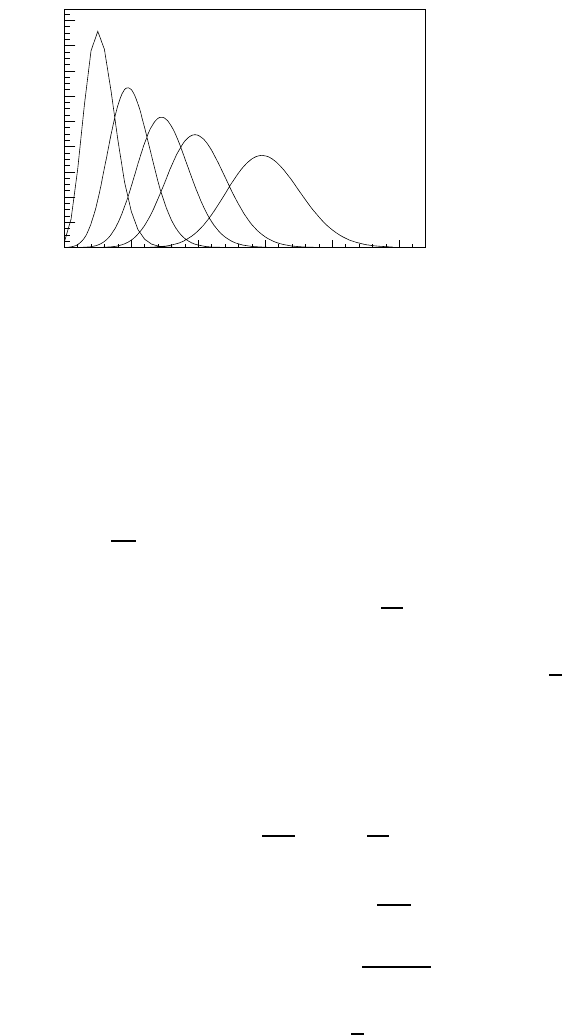
obtained from a detection system and µ>0 is the mean. Fig.9.3.3 depicts this

distribution for diﬀerent values of µ. It is apparent that the width of the distribution

increases with µ, which indicates that the uncertainty in measurement increases with

an increase in the value of x.

Let us now apply the maximum likelihood method to determine the best estimate

of mean of a set of n measurements assuming that the underlying process is Pois-

son in nature. The best way to do this is to use the maximum likelihood method

we outlined earlier and applied in the previous section while discussing the Bino-

mial distribution. Since Poisson distribution is a discrete probability distribution

therefore its likelihood function for a set of n measurements can be written as

L(µ)=

i=1

f(x

,µ)

i=1



−µ



−nµ

!...x

(9.3.32)

538 Chapter 9. Essential Statistics for Data Analysis

0 1020304050

0.02

0.04

0.06

0.08

0.1

0.12

0.14

0.16

0.18

=5.5µ

=10µ

=15µ

=30µ

=20µ

Figure 9.3.3: Poisson probabil-

ity density for diﬀerent values of

µ. The width of the distribu-

tion, a reﬂection of the uncer-

tainty in the measurement, in-

creases with increase in µ.

The log likelihood function of L(µ)is

l ≡ ln(L)=





i=1



ln(µ) − nµ − ln(x

!...x

!). (9.3.33)

Following the maximum likelihood method (∂l/∂µ =0)weget

∂

∂µ





i=1



ln(µ) − nµ − ln(x

!...x



∗



i=1

− n =0

∗



i=1

. (9.3.34)

This shows that the simple mean is the most probable value of a Poisson distributed

variable. To determine the error in µ, we ﬁst take second derivative of the log

likelihood function and then substitute it in equation 9.3.22.

∂

∂µ

= −



i=1

µ =



−

∂

∂µ



−1/2



∗2

i=1



1/2





i=1



1/2

(9.3.35)

This is one of the most useful results of the Poisson distribution. It implies that if

we make one measurement, the statistical error we should expect in it would simply

9.3. Probability 539

be the square root of the measured quantity. For example, if we count the number of

γ-ray photons coming from a radioactive source using a GM-tube and get a number

N, the statistical error we should expect will simply be

√

N. Fortunately, most of

the processes we encounter in the ﬁeld of radiation detection and measurement, such

as activity of a radioisotope, photoelectric eﬀect, and electron multiplication in a

PMT tube, can all very well be described by Poisson statistics.

D.3 Normal or Gaussian Distribution

The normal distribution was originally developed as an approximation to the bi-

nomial distribution. Its usefulness was soon recognized by scientists and soon it

became one of the most commonly used probability distributions in not only these

ﬁelds but also in other sciences. The utility of normal distribution can be appre-

ciated by noting an amazing property of most of the physical processes that their

random variables can be safely approximated to be distributed normally. Therefore

a common practice is to assume that a random variable having unknown distribu-

tion can be deﬁned by a normal distribution. This property of random variables

is actually the result of the so called central limit theorem, which states that the

mean of any set of variables with any distribution tend to the normal distribution

provided their mean and variance are ﬁnite. Although the term normal distribution

is very commonly used, still some scientists prefer to call it Gaussian distribution.

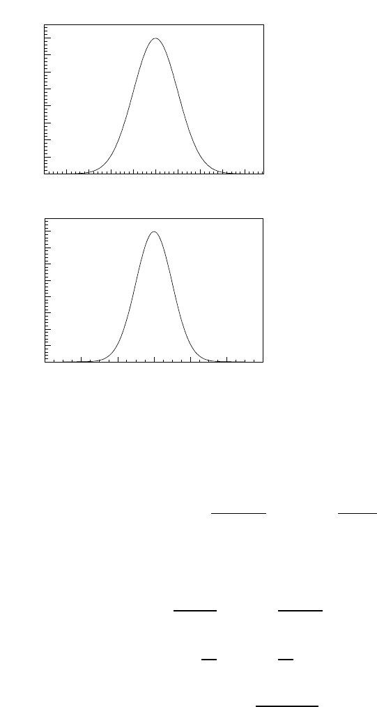
Gaussian distribution has a bell-shaped curve (see Fig.9.3.4) and is deﬁned for a

variable x in the domain x ∈ (−∞, ∞)by

f(µ; x)=

√

2π

−(x−µ)

/2σ

, (9.3.36)

where µ and σ are the mean and standard deviation of the distribution respectively.

Both µ and σ are ﬁnite for a normally distributed variable.

If we substitute µ =0andσ

= 1 in the above equation, we obtain the so called

standard normal distribution with a probability density function given by

P (x)=

√

2π

−x

. (9.3.37)

This is simply a special kind of Gaussian distribution having a symmetric bell shaped

curve centered at x = 0 (see Fig.9.3.4). In fact by changing the variables, any

normal distribution can be easily converted into a standard normal distribution (see

Example below).

Let us now apply our maximum likelihood method to compute the most probable

value and its accuracy assuming the variable to be Gaussian distributed. Suppose

we make N measurements of a variable and represent the result by x

.Eachofthese

measurements will have its own error σ

. Then according to equation 9.3.19, the

likelihood function is given by

L(µ)=

i=1

√

2π

−(x

−µ)

/2σ

(9.3.38)

In order to apply the condition 9.3.23, we rewrite the above equation in the form

L(µ)=

i=1

−(x

−µ)

/2σ

)(σ

−1

)(2π)

−1/2

(9.3.39)

540 Chapter 9. Essential Statistics for Data Analysis

0 5 10 15 20 25 30 35 40 45

0.01

0.02

0.03

0.04

0.05

0.06

0.07

0.08

-4 -2 0 2 4

0.05

0.1

0.15

0.2

0.25

0.3

0.35

0.4

Figure 9.3.4: (a) Gaussian dis-

tribution for µ =25andσ =

5. (b) Standard normal distri-

bution having µ =0andσ =

1. With proper change of scale,

any Gaussian distribution can be

transformed into a standard nor-

mal distribution.

Taking the natural logarithm of both sides of this equation gives

ln(L)=



i=1



−

−µ)

2σ

− ln(σ

) −

ln(2π)



. (9.3.40)

The maximum likelihood solution is then obtained by diﬀerentiating this equation

with respect to µ and equating the result to zero. Hence we get

∂ ln(L)

∂µ

∗



i=1

− µ

∗

= 0 (9.3.41)

⇒



i=1

∗



i=1

⇒ µ

∗

i=1

, (9.3.42)

where w

=1/σ

. Hence the most probable value is simply the weighted mean with

respective inverse variances or errors as weights. If we assume that each measure-

ment has the same amount of uncertainty or error then using σ

= σ the maximum

9.3. Probability 541

likelihood solution will become

∗

i=1

/σ

i=1

(1/σ)



i=1

, (9.3.43)

which is nothing but the expression for calculating simple mean. Hence we have

found that calculating mean by this method require that the variable is distributed

normally and that each measurement has the same error associated with it. Measur-

ing activity of a radioactive source falls into this category provided all the conditions

including the state of the detector does not change with time.

Let us now try to calculate the error in the calculation of the solution we just

obtained. Note that we are interested in ﬁnding out the spread of µ about µ

∗

and not

the errors in individual measurements. To do this we make use of the argument that

for large number of measurements (N →∞), L(µ) approaches a normal distribution.

Hence we can write

L(µ)=

√

2π

−(µ−µ

∗

)

/2σ

(9.3.44)

Here the subscript t in σ

is meant to diﬀerentiate the standard deviation of µ from

that of x. Again the condition 9.3.23 can be used to obtain the maximum likelihood

solution for this distribution. We ﬁrst take the natural logarithm of both sides of

the above equation to obtain

ln(L)=ln



−(µ−µ

∗

)

/2σ



(σ

)

−1

(2π)

−1/2



= −

(µ − µ

∗

)

2σ

−ln(σ

) −

ln(2π)

. (9.3.45)

Diﬀerentiating this twice with respect to µ

∗

gives

∂ ln(L)

∂µ

∗

µ − µ

∗

⇒

∂

ln(L)

∂µ

∗2

= −

. (9.3.46)

Hence the error in calculation of µ,isgivenby

µ = σ



−

∂

ln(L)

∂µ

∗2



−1/2

. (9.3.47)

This general expression for computing errors is of central importance in likelihood

method and is extensively used in data analysis. Let us now use this expression to

derive the expression for the total error in measurements when each measurement

is characterized by its own error σ

. This can be done by diﬀerentiating equation

542 Chapter 9. Essential Statistics for Data Analysis

9.3.41 again with respect to µ

∗

and substituting the result in the above expression.

∂

∂µ

= −



i=1

⇒



i=1

(9.3.48)

This expression represents the law of combination of errors, which states that for

repeated measurements of a normally distributed variable having errors σ

,thein-

verse of the total error in the calculation of mean is equal to the sum of inverse of

individual measurement errors.

Unfortunately, in a number of practical problems, an analytic determination of

µ is not possible. In such cases one tries to ﬁnd the value of the likelihood function

at each point by iterating µ (or more accurately, by trying diﬀerent values of µ).

The points thus obtained are then plotted and the likelihood function is obtained

by performing the best ﬁt through the points. In most cases with large number of

data points the likelihood function is Gaussian like. If it isn’t, one must perform a

weighted average to determine the error function, that is

∂

ln(L)

∂µ



∂

ln(L)

∂µ

Ldµ



Ldµ

. (9.3.49)

This is an important relation since it can be used to show that (see problems at the

end of the chapter) the maximum likelihood error in µ can be evaluated from

µ =







∂L

∂µ





1/2

, (9.3.50)

where N is the number of measurements. An interesting aspect of this result is

that it allows one to determine the number of measurements necessary to obtain a

particular value of the parameter µ with a certain accuracy, that is

N =

(µ)





∂L

∂µ



dx. (9.3.51)

D.4 Chi-Square (χ

) Distribution

-distribution is one of the most extensively used probability distributions to per-

form goodness-of-ﬁt tests, which we will discuss later in the chapter. It is deﬁned as

f(x; n)=

n/2−1

−x/2

n/2

Γ(n/2)

, (9.3.52)

where in order to avoid confusion due to the exponent 2 of χ

we have represented it

by x. Γ() is the gamma function and x ≥ 0. The tables as well as analytical forms of

gamma functions can be found in standard texts of statistics and mathematics. The

parameter n in the above deﬁnition is called the degrees of freedom of the system.

The meaning of this term can be understood by looking at the deﬁnition of x or χ

9.3. Probability 543

Suppose we have m independent normally distributed random variables u

having

theoretical means µ

and variances σ

. χ

is then deﬁned as

≡ x =



i=1

− µ

)

. (9.3.53)

The parameter n in the deﬁnition of the χ

probability distribution is then related to

the number of independent variables in this equation. For large n the χ

distribution

reduces to the Gaussian distribution with mean µ = n and variance σ

=2n.

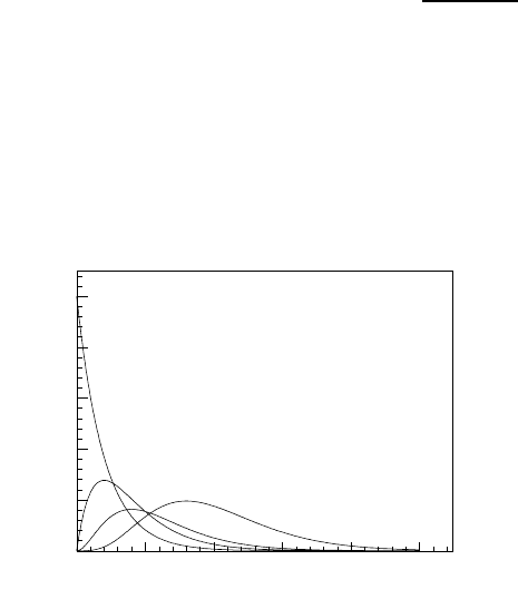
Fig.9.3.5 shows the shapes of the chi-square distribution for diﬀerent degrees of

freedom. As n increases, the distribution assumes a shape that becomes more and

more like a Gaussian or normal distribution.

0 5 10 15 20 25

0.1

0.2

0.3

0.4

0.5

n=2

n=5

n=7

n=10

Figure 9.3.5: χ

probability den-

sity functions for diﬀerent degrees

of freedom n. The shape of the

distribution approaches that of

a Gaussian distribution with in-

creasing n.

To understand the utility of this distribution function, let us have a closer look

at the deﬁnition 9.3.53. The numerator in this equation represents the deviations of

the normally distributed variable u

from its theoretical means at each data point

while the denominator represents its expected standard deviations. In other words

the numerator and denominator are the actual and expected deviations respectively.

If the data u

is really Gaussian distributed, then ideally the actual deviation should

be equal to the expected one. However in real data there are always ﬂuctuations

and consequently these deviations are not equal. The χ

probability density function

9.3.52 actually tells us how the probability of this deviation is distributed. Hence

this distribution function can be used to judge the data against a hypothetical mean.

We will learn more about this when we discuss the goodness-of-ﬁt tests later in the

chapter.

D.5 Student’s t Distribution

Student’s t distribution is a widely used probability distribution. It forms the ba-

sis of Student’s t-test, which we will discuss later in the chapter. To deﬁne this

544 Chapter 9. Essential Statistics for Data Analysis

distribution, let us ﬁrst write

z =



i=1

and t =



z/n

for n independent Gaussian variables having 0 mean and 1 variance. The variable

z in this expression follows the χ

-distribution we deﬁned above and the variable t

follows Student’s t distribution with n degrees of freedom deﬁned by

f(t; n)=

√

nπ

Γ[(n +1)/2]

Γ(n/2)





−(n+1)/2

, (9.3.54)

where Γ is the familiar gamma function, the variable t can take any value (−∞ <

t<∞), and n can be a non-integer.

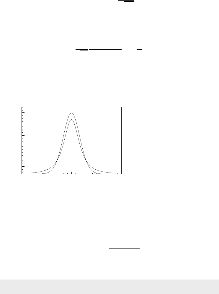
The Student’s t distribution looks very similar to Gaussian distribution. For

small n, however it has wider tails, which approach that of a Gaussian distribution

with increasing n.

-4 -2 0 2 4

0.05

0.1

0.15

0.2

0.25

0.3

0.35

0.4

n=2

n=30

Figure 9.3.6: Student’s t distri-

bution for two values of degrees

of freedom n.Asn increases

the tails of the distribution ap-

proaches that of a Gaussian dis-

tribution.

D.6 Gamma Distribution

For a Poisson process the distance in x from any starting point to the k

h event

follows Gamma distribution given by

f(x; λ, k)=

k−1

−λx

Γ(k)

, (9.3.55)

with 0 <t<∞ and k can be a noninteger.

For λ =1/2andk = n/2 it reduces to the χ

-distribution we deﬁned above.

Using Maximum Likelihood Method

9.3. Probability 545

Now that we have learned all the basics of maximum likelihood methodology, we

are ready to use it in practical situations. By practical situations we mean the real

cases corresponding to distributions that are not perfectly described by the standard

distribution functions we just studied. Let us suppose we have a variable x,whose

probability distribution function can be written as

p(x, k)=ke

−kt

where k is a constant. Suppose we take 4 measurements of the parameter t: t =

12, 14, 11, 12. What we want to do is to use the maximum likelihood method to

compute the value of the constant k. To do this we ﬁrst need to determine the

maximum likelihood function. According to equation 9.3.19, this is give by

L(k)=

i=1

−kt

= e

−k

)

= k

−49k

Now we take the natural logarithm of this function.

ln(L)=4ln(k) − 49k

According to the maximum likelihood method, diﬀerentiating the above function

with respect to k and equation the result to zero gives the required maximum like-

lihood estimate of k.

∂ ln(L)

∂k

⇒

− 49 = 0

⇒ k =

Let us now look at another example. This time we want to know how many

measurements we must make so that the parameter k =0.21 of the distribution

f(x, k)=kx ; x ∈ (0, 1),

can be determined with an accuracy of 5%. That is, the relative error in k =0.21

k

=0.05. (9.3.56)

This can easily be done by using equation 9.3.51, which for our case becomes

N =

(k)





∂f

∂k



dx.