Ahmed S.N. Physics and Engineering of Radiation Detection

Подождите немного. Документ загружается.

546 Chapter 9. Essential Statistics for Data Analysis

With f = kx,weget



∂f

∂k



= x

⇒



∂f

∂k



⇒





∂f

∂k



dx =

Substituting this in the above relation for N gives

N =

(k)

But we have k =0.21 and k =0.05k =0.0105, which gives

N =

(0.0105)

(2)(0.21)

=2.1 × 10

9.4 Conﬁdence Intervals

Suppose we have a rough idea of the activity level in a radiation environment and

we use this information to estimate the dose that we expect a radiation worker to

receive while working there for some speciﬁc period of time. The problem with this

scheme is that there are a number of uncertainties involved in the computations,

such as level of actual activity, its space dependence (the radiation sources might

not be isotropic), and its variation with time. In such a situation what can be

done is to deﬁne a conﬁdence interval within which the value is expected to lie with

a certain probability. For example, we can say that there is 90% probability that

the person will receive a dose of somewhere between 10-20 mrem.Herewehave

two parameters that we are reporting: the conﬁdence interval and its associated

probability. The choice of a conﬁdence interval is more or less arbitrary, although

generally it is based on some rationale, such as our rough estimation based on

some known parameters (in our example, we might have gotten a value of 15 mrem

and then decided to give ourselves a leverage of ±5 mrem to compensate for any

uncertainty in the calculations.). The probability, on the other hand, depends on

the conﬁdence interval and the probability distribution.

If the probability distribution of a variable x (such as dose) is given by L(x), then

the probability that x lies between x

and x

is given by

P (x

<x<x



L(x)dx



∞

−∞

L(x)dx

. (9.4.1)

9.4. Conﬁdence Intervals 547

If the function L(x) is normalized, then the denominator becomes 1 and the

probability is simply given by

P =



L(x)dx. (9.4.2)

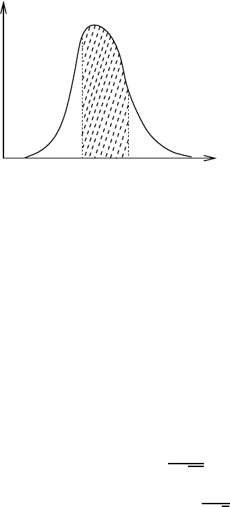
This probability is actually the area under the curve of L(x) versus x between

the points x

and x

and therefore depends on the choice of the conﬁdence interval

(see Fig.9.4.1).

(x)

Figure 9.4.1: The probability that a

value x lies within a conﬁdence interval of

) is obtained by dividing the area

under the curve (shaded section) by the

total area. If the distribution is nor-

malized then the denominator will be 1

and the shaded area will simply be the

required probability. This probability,

therefore, depends on the choice of con-

ﬁdence interval. In practice, the proba-

bility is ﬁrst selected and then the conﬁ-

dence interval is obtained from the cumu-

lative distribution function of the proba-

bility distribution.

We saw above that the choice of conﬁdence interval is arbitrary while the prob-

ability depends on it. Therefore one would assume that the interval is ﬁrst chosen

and then the probability is calculated. However the general practice is quite the

opposite. If it is known that the process under consideration has a certain probabil-

ity distribution then the probability is ﬁrst chosen and then the conﬁdence interval

is deduced from some available tables or curves. For example, for Gaussian dis-

tribution, which is the most commonly used distribution, the tables of probability

integrals are used to ﬁnd the conﬁdence intervals.

Let us now take a look at the example of a normally distributed variable x

having mean µ and variance σ

. We are interested in ﬁnding the probability that

the measured value lies between µ − δx and µ + δx. This probability, according to

the deﬁnition above, can be evaluated from

P =

√

2π



µ+δx

µ−δx

−(x−µ)

/2σ

= erf



δx

√



. (9.4.3)

Here erf (u)istheerror function of u, whose values are available in tabulated

form in standard texts. To get a feeling of what diﬀerent values of P would mean

548 Chapter 9. Essential Statistics for Data Analysis

with respect to σ,welookatsometypicalvalues.

P (µ − σ<x<µ+ σ)=0.6827

P (µ − 2σ<x<µ+2σ)=0.9545

P (µ − 3σ<x<µ+3σ)=0.9973

What these values essentially show is that if the data can be represented by

a perfect Gaussian distribution, then we can be only 68.27% sure that the next

measurement will lie within the range µ ±σ. However if we wanted to be more than

99% sure about this we will have to stretch the range to around 3σ on both sides of

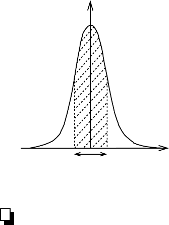
the distribution. Fig.9.4.2 explains this concept in graphical form.

f(x)

Figure 9.4.2: Conﬁdence interval of a stan-

dard Gaussian distribution. The shaded area

represents the probability that the next mea-

surement of x will lie within the interval µ−σ<

x<µ+ σ. For a perfect Gaussian distribution

this turns out to be 0.6827 meaning that one

could be up to 68.27% sure that the value will

not be out of these bounds.

9.5 Measurement Uncertainty

There is always some uncertainty associated with a measurement no matter how

good our measuring device is and how carefully we perform the experiment. There

are diﬀerent types of uncertainties associated with any measurement but they can

be broadly divided into two categories: systematic and random.

9.5.A Systematic Errors

All measurements, direct or indirect, are done through some type of measuring de-

vice. Since there is no such thing as a perfect device, therefore one should expect

some error associated with the measurement. This type of error falls into the cate-

gory of systematic errors, which refer to the uncertainties in the measurement due

to the measurement procedures and devices. Unfortunately it is not always easy

to characterize systematic errors. Repeating the measurements does not have any

eﬀect on them since they are not random. In other words, systematic errors are not

statistical in nature and therefore can not be determined by statistical methods.

The good thing is that the systematic uncertainties can be minimized by modi-

fying the procedures and using better devices. For example, one can use a detector

9.5. Measurement Uncertainty 549

having better accuracy or, in case of a gas ﬁlled detector, improve on its accuracy by

using a more eﬃcient gas mixture. Similarly easy steps can be taken to decrease the

systematic uncertainties associated with readout electronics. An obvious example of

that would be the use of an ADC having better resolution. Another way to decrease

the systematic uncertainty is to properly calibrate the system.

Systematic uncertainties are system speciﬁc and therefore there is no general

formula that could be used for their characterization. It is up to the experimenter

to carefully determine these errors and faithfully report them in the ﬁnal results.

9.5.B Random Errors

Random errors refer to the errors that are statistical in nature. For example, the

radioactive decay is a random process. Even though we know the average rate of

decay of a sample, we can not predict when the next decay will happen. This implies

that there is an inherent time uncertainty associated with the process. Similarly the

production of charge pairs in a radiation detector by passing radiation is also a

random process (see chapter 2). We can say that on the average how many charge

pairs will be produced by a certain amount of deposited energy but we can not

associate an absolute number to it. Such uncertainties that are inherent to the

process and are statistical in nature are categorized as random uncertainties.

Fortunately most physical processes are Poisson in nature. This makes is fairly

easy to estimate the random error associated with a measurement. The random

error associated with a measurement during which N counts were recorded, is given

stat

√

N. (9.5.1)

For example, let us suppose that we measure the activity of a radioactive sample

by taking three consecutive readings by a single channel analyzer/counter: 2452,

2367, 2398. The absolute random errors associated with these measurements will

be:

stat,1

√

2452 = 49.52

stat,2

√

2367 = 48.65

stat,3

√

2398 = 48.97

9.5.C Error Propagation

Let us suppose we perform an experiment and make N independent measurements

each having uncertainty δx

and standard deviation sigma

. We then use these

measurements to evaluate some function u = f (x

, ..., x

). The question is: how

can we estimate the standard deviation and error in the quantity we thus determine?

This is where the error propagation formulae come into play, according to which the

combined variance and standard error in the function u can be evaluated from



∂f

∂x





∂f

∂x



+ .... +



∂f

∂x



(9.5.2)

and δ





∂f

∂x



δx



∂f

∂x



δx

+ .... +



∂f

∂x



δx



1/2

. (9.5.3)

550 Chapter 9. Essential Statistics for Data Analysis

These general relations can be used to derive formulae for speciﬁc functions as

shown below.

C.1 Addition of Parameters

Suppose we have u = x

+ x

+ .... + x

. In this case the derivatives of u = f (x)

will be given by

∂f

∂x

∂f

∂x

= .... =

∂f

∂x

=1. (9.5.4)

Equation 9.5.3, then reduces to



δx

+ δx

+ .... + δx



1/2

, (9.5.5)

which states that the total error in the measurement will simply be equal to the

square root of the sum of individual errors squared.

Note that the above formula also holds if the some or all of the parameters have

negative signs. In other words, the formula remains the same whether the parameters

are added or subtracted in the function.

C.2 Multiplication of Parameters

Let us now see how the errors propagate if the function has the multiplicative form.

For simplicity we will restrict ourselves to two variables, that is, we will assume that

u = x

. In this case the derivatives of u = f (x) will be given by

∂f

∂x

= x

(9.5.6)

and

∂f

∂x

= x

. (9.5.7)

Substituting these values into equation 9.5.3 gives





δx





δx





1/2

. (9.5.8)

The generalized form of this equation for N parameters is given by





δx





δx



+ .... +



δx





1/2

. (9.5.9)

Note that here δ

/u refers to relative error. For absolute error this must be multiplied

by u. What the above formula tells us is that the relative error in the measurement of

N independent measurements is simply the square root of the sum of the individual

relative errors squared.

The reader can verify that the above formula does not change its form in case of

division. For example, the error in u = x

can be determined from the above

formula without any modiﬁcations.

9.6. Conﬁdence Tests 551

9.5.D Presentation of Results

Now that we know how to calculate errors associated with parameters by using errors

in individual measurements, we should discuss how to present our ﬁnal results. We

saw earlier that there are basically two classes of errors: systematic and random.

Though it is a common practice to combine both errors together in the ﬁnal result

but a better approach, as adopted by many careful experimenters, is to explicitly

state them separately. For example, the result of an experiment might be represented

at 1σ conﬁdence as

ξ = 205.43 ±6.13

syst

± 14.36

rand

where the superscripts syst and rand stand for systematic and random errors respec-

tively.

A word of caution here. By looking at the above numbers, one might naively

conclude that all the values would lie between 205−6.13−14.36 and 205+6.13+14.36.

This is not really true. Earlier in the chapter we discussed the conﬁdence intervals

and we saw that, for normally distributed data, a 1σ uncertainty guarantees with

only about 68% conﬁdence that the result lies within the given values (that is,

between

ξ −σ and

ξ + σ). For higher conﬁdence, one must increase the σ-level.For

example, for a 99% conﬁdence, the above result will have to be written as

ξ = 205.43 ±6.13

syst

± 43.08

rand

where we have multiplied the random error of 1σ by a factor of 3. Note that, since

systematic uncertainty does not depend on statistical ﬂuctuations, there is no need

to multiply it by any factor. Now we can say with 99% conﬁdence that the value of

the parameter lies between 205 − 6.13 − 43.08 and 205 + 6.13 + 43.08.

9.6 Conﬁdence Tests

Computing diﬀerent quantities from a data set obtained from an experiment is

helpful in understanding the characteristics of the system but if we have a certain

bias about the behavior of the system we might also want to judge the data against

our hypothesis. This judgment can be qualitative, such as just a visual sense of how

the data looks like with respect to the expectation, or quantitative, which is the

subject of the discussion here.

To judge a data sample quantitatively against a hypothesis we perform the so

called conﬁdence or goodness-of-ﬁt test. For this we ﬁrst deﬁne a goodness-of-ﬁt

statistic by taking into account both the data and the hypothesis. The idea is

to have a quantity whose probability of occurrence could tell us about the level of

agreement between the data and the hypothesis. Of course the choice of this statistic

is arbitrary but several standard functions have been generated that can be applied

in most of the cases. Before we look at some of these functions, let us ﬁrst see how

the general procedure works.

Let us represent the goodness-of-ﬁt statistic by t such that its large values corre-

spond to poor agreement with the hypothesis h. Then the p.d.f g(t|h)canbeused

to determine the probability p of ﬁnding t in a region starting from the experimen-

tally obtained value t

up to the maximum. This is equivalent to evaluating the

552 Chapter 9. Essential Statistics for Data Analysis

cumulative distribution function

p ≡ 1 − P (t

)=1−



−∞

g(t|h)dt or

p =



∞

g(t|h)dt (9.6.1)

A single value of p, however, does not tell us much about the agreement between

data and hypothesis because at each data point the level of agreement could be

diﬀerent. The trick is to see how the value of p is distributed throughout its range,

that is, between 0 and 1. Of course if there is perfect agreement, the distribution

will be uniform.

Let us now take a look at some of the commonly used goodness-of-ﬁt statistics.

9.6.A Chi-Square (χ

)Test

This is perhaps one of the most widely used goodness-of-ﬁt statistic. In the following

we outline the steps needed to perform the test.

1. The foremost thing to do is to construct a hypothesis, which has to be tested.

This hypothesis should include a set of values µ

that we expect to get if we

perform measurements and obtain the values u

. These set of values may have

been derived from a known distribution that the system is supposed to follow.

2. Decide on the number of degrees of freedom. If we take N measurements, the

degrees of freedom are not necessarily equal to N because there may be one

or more relations connecting the measured values u

.Ifthenumberofsuch

relations are r, then the degrees of freedom will be given by ν = N −r.

3. Using the measured values u

, compute a sample value of χ

from the relation

9.3.53



i=1

− µ

)

4. Compute the normalized χ

,thatis,χ

/ν.

5. Decide on the acceptable signiﬁcance level p, which represents the probability

that the data is in agreement with the hypothesis or not. A commonly chosen

value of p is 0.05, which gives a conﬁdence of 95%.

6. Determine the value of χ

ν,p

at which p is equal to the chosen value. This means

evaluating the integral

p =



∞

ν,p

f(x)dx (9.6.2)

for χ

ν,p

(see also equation 9.6.1). f(x)isofcoursetheχ

probability den-

sity function. The solution to this equation requires numerical manipulations,

which can be done, for example by employing the Monte Carlo integration

technique. However this is not generally done since there are tables and graphs

available that can be used to deduce the values of χ

ν,p

with respect to p and ν.

9.6. Conﬁdence Tests 553

7. Compare χ

/ν with χ

ν,α

/ν.

Let us now see what we can infer from this comparison.

 Case-1, χ

/ν  χ

ν,α

/ν: We are up to α ×100% conﬁdent that our hypothesis

was correct.

 Case-2, χ

/ν > χ

ν,α

/ν: This may mean one of the following.

1. The model we have chosen to represent the system is not adequate.

2. The model is adequate but there are some bad data points in the sample.

It takes only a few large excursions in the data that are far away from the

mean to yield a large value of chi-square. Care should therefore be taken

to ensure that proper ﬁltration of the data is performed to eliminate such

data points.

3. The data values are not uniformly distributed about their means. The is

the most troubling scenario, since it would mean that this goodness-of-ﬁt

method is not really applicable and we should either resort to some other

method or look closely at the data to ﬁnd out if just a few values are

causing this deviation from the normal distribution. Generally, discarding

a few data points does the trick.

 Case-3, χ

/ν < χ

ν,α

/ν: This means that the squares of the random normal

deviates are less than expected, a situation that demands as much attention as

the previous one. The following possibilities exist for this case.

1. The expected means were overestimated. This does not mean that the

model was wrong.

2. There are a few data points that have caused the chi-square value to

become too small.

9.6.B Student’s t Test

Student’s t test is the most commonly used method of comparing the means of

two low statistics data samples. To perform the test, ﬁrst the following quantity is

evaluated.

t =

| ¯x

− ¯x

(9.6.3)

Here ¯x

and ¯x

represent the means of ﬁrst and second datasets and σ

is the

standard deviation of the diﬀerence between the two means. It can be computed

from





1/2

, (9.6.4)

where σ

and σ

are the standard deviations of the two datasets having N

and N

number of data points. Note that here what we have done is to simply taken the

square root of the sum of the standard errors associated with each dataset.

The next step is to compare the calculated t-value with the tabulated one. The

tabulated values, derived from the Student’s t distribution we presented earlier, are

554 Chapter 9. Essential Statistics for Data Analysis

generally given for diﬀerent degrees of freedom and levels of signiﬁcance. The total

degrees of freedom for the dataset are given by

ν =(N

− 1) + (N

− 1)

= N

+ N

− 2. (9.6.5)

The choice of level of signiﬁcance depends on the level of conﬁdence one intends to

have on the analysis. If one chooses a value of 0.05 and the calculated t value turns

out to be less than the tabulated one, then one could say with 95% conﬁdence that

the means are not signiﬁcantly diﬀerent.

Example:

An ionization chamber is used to measure the intensity of x-rays from an

x-ray machine. The experiment is performed at two diﬀerent times and yield

the following values (arbitrary units).

Measurement-1: 380, 398, 420, 405, 378

Measurement-2: 370, 385, 400, 419, 415, 375

Perform Student’s t test at 95% and 99% conﬁdence levels to see if the means

of the two measurements are signiﬁcantly diﬀerent from each other.

Solution:

First we compute the means of the two datasets.

¯x



i=1

1,i

= 396.2

¯x



i=1

2,i

= 394

Next we determine the standard deviations of the two means.

− 1



i=1

1,i

− ¯x

)

=17.61

− 1



i=1

2,i

− ¯x

)

=20.59

9.7. Regression 555

The standard deviation of the mean is given by





1/2



17.61

20.59



1/2

=11.52.

Now we are ready to compute the t value.

t =

|396.2 −394|

11.52

=0.191

To compare this t value with the tabulated values we must ﬁrst determine the

degrees of freedom of the dataset. This is given by

ν = N

+ N

−2

=5+6− 2=9.

For a 95% conﬁdence level and 9 degrees of freedom the tabulated t value is

2.26. And for a 99% conﬁdence level the tablulated t value is 1.83. Since

both of these values are greater than the calculated t value of 0.19, therefore

we can say with at least 99% conﬁdence that the two dataset means are not

signiﬁcantly diﬀerent.

9.7 Regression

Regression analysis is perhaps the most widely used technique to draw inferences

from experimental data. The basic idea behind it is to ﬁt a function that closely

represents the trend in the data. The function can then be used to make predictions

about the variables involved.

Fitting a function to the data through regression analysis is not always a very

pleasant experience, specially if the data shows variations that can not be charac-

terized by standard functions, such as polynomial, exponential, or logarithmic. The

easiest form of regression analysis is the simple linear regression, which we will dis-

cuss in some detail now. Later on we will look at other kinds of regression analysis.

9.7.A Simple Linear Regression

Simple linear regression refers to ﬁtting a straight line to the data. The ﬁtting

is mostly done using a technique called least square ﬁtting. To understand this

technique, let us start with the equation of a straight line

y = mx + c, (9.7.1)

where m is the slope of the line and c is its y-intercept. Since slope and y-intercept

determine the orientation and position of the straight line on the xy-plot, therefore