Atkinson K. An Introduction to Numerical Analysis
Подождите немного. Документ загружается.

.....
/
GAUSSIAN QUADRATURE
279
along with the true error. The error bound
is
of approximately the same
magnitude as the true error.
Discussion of Gauss-Legendre quadrature We begin by trying
to
make the
error term
(5.3.29) more understandable. First define
M =
m
Max
-lsxsl
m!
m~O
(5.3.34)
For a large class of infinitely differentiable functions f on [
-1,
1],
we
have
Supremumm;;,;oMm
<
oo.
For example, this will be true if
f(z)
is
analytic on the
region
R of the complex plane defined by
R = { z:
lz
- xl
~
1 for some
x,
-1
~
x
~
1}
With many functions,
Mm
~
0
as
m
~
oo,
for example,
f(x)
=ex
and
cos(x).
Combining (5.3.29) and (5.3.34),
we
obtain
n~1
(5.3.35)
and the size of
en
is essential in examining the speed of convergence.
The term
en
can be made more understandable by estimating it using Stirling's
formula,
which
is
true in a relative error sense
as
n
~
oo.
Then
we
obtain
as
n~oo
(5.3.36)
This
is
quite a good estimate. For example, e
5
= .00293, and (5.3.36) gives the
estimate
.00307. Combined with (5.3.35), this implies
(5.3.37)
which
is
a correct bound in an asymptotic sense
as
n
~
oo.
This shows that
En(/)
~
0 with an exponential rate
of
decrease
as
a function
of
n. Compare this
with the polynomial rates of
1jn
2
and
1/n
4
for the trapezoidal and Simpson
rules, respectively.
In order to consider integrands that are not infinitely differentiable,
we
can use
the
Peano kernel form of the error, just as in Section
5.1
for Simpson's and the
trapezoidal rules.
If
f(x)
is
r times differentiable on [
-1,
1],
with J<'>(x)
integrable on [
-1,
1],
then
r
n
>-
2
(5.3.38)
!
i
'
280
NUMERICAL INTEGRATION
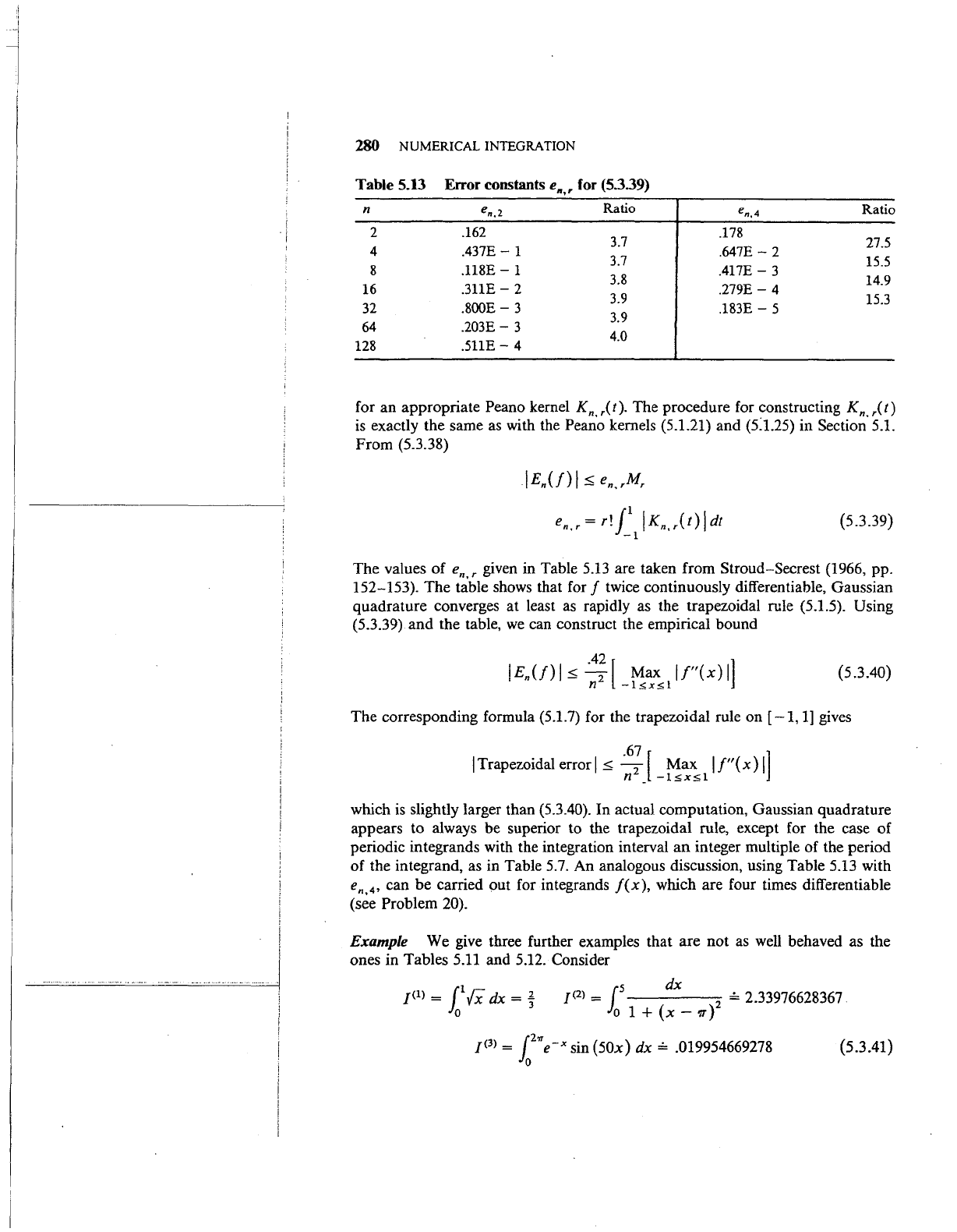
Table 5.13
Error constants
e,,,
for (5.3.39)
n
en,2
Ratio
en,4
Ratio
2
.162
.178
3.7
27.5
4
.437£-
1
.647£-2
8
.118£-
1
3.7
.417£-3
15.5
16
.311£-
2
3.8
.279£-4
14.9
32
.800£-
3
3.9
.183£-
5
15.3
3.9
64
.203£-
3
4.0
128
.511£-
4
for an appropriate Peano kernel Kn.r(t). The procedure for constructing
Knjt)
is
exactly the same
as
with the Peano kernels (5.1.21) and (5:1.25) in Section 5.1.
From (5.3.38)
lEn(!)
I~
en,rMr
en.
r = r! F I K
n.
r (
l)
I dt
-1
(5.3.39)
The values of
en.,
given in Table 5.13 are taken from Stroud-Secrest (1966, pp.
152-153). The table shows that for f twice continuously differentiable, Gaussian
quadrature converges at least as rapidly as the trapezoidal rule
(5.1.5). Using
(5.3.39) and the table,
we
can construct the empirical bound
.42 [ ]
lEn(!)
I~
-
2
Max
lf"(x)
I
n
-l!>x!>l
(5.3.40)
The corresponding formula (5.1.7) for the trapezoidal rule on [
-1,
1] gives
.67 [ ]
I Trapezoidal error I
~
-;;z_
_
i'!:";;
1
I!" (
x)
I
which
is
slightly larger than (5.3.40). In actual computation, Gaussian quadrature
appears to always be superior to the trapezoidal rule, except for the case of
periodic integrands with the integration interval
an
integer multiple of the period
of
the integrand, as in Table 5.7. An analogous discussion, using Table 5.13 with
en,
4
,
can be carried out for integrands
j(x),
which are four times differentiable
(see
Problem 20).
Example We give three further examples that are not
as
well
behaved as the
ones in Tables
5.11 and 5.12. Consider
5
dx
J(
2
)
= 1 2
~
2.33976628367
o 1 +
(x-
'17)
[2'1T
J<
3
l
=
Jn
e-x
sin
(50x)
dx
~
.019954669278
0
(5.3.41)
l
.......•......
\
GAUSSIAN
QUADRATURE
281
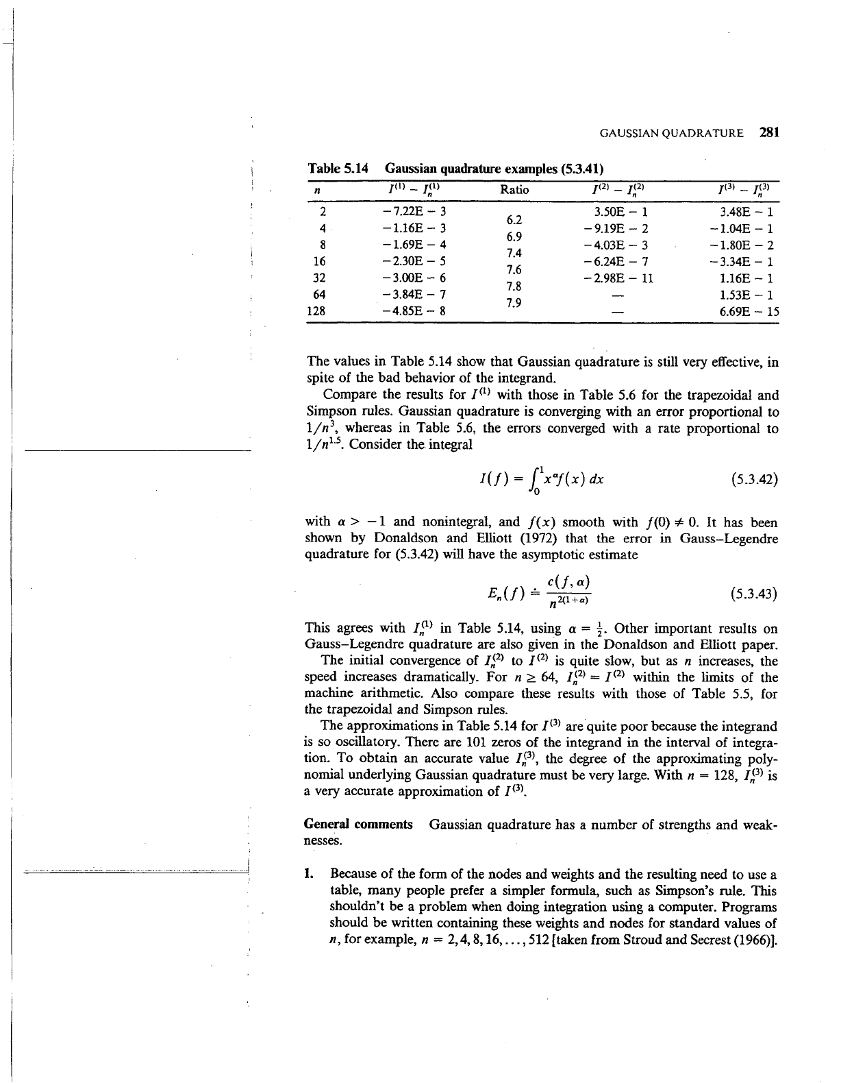
Table 5.14 Gaussian quadrature examples (5.3.41)
n
2
4
8
16
32
64
128
JOl
_
/~ll
-7.22£-
3
-1.16£-
3
-1.69£-4
-2.30£-
5
-3.00£-
6
-3.84£-
7
-4.85£-
8
Ratio
6.2
6.9
7.4
7.6
7.8
7.9
/(2)-
/~2)
J<3l
-
/~3)
3.50£-
1
3.48£-
1
-9.19£-
2
-1.04£-1
-4.03£-
3
-1.80£-
2
-6.24£-
7
-3.34£-
1
-2.98£-
11
1.16£-
1
1.53£-
1
6.69£-
15
The values in Table 5.14 show that Gaussian quadrature
is
still very effective, in
spite of the bad behavior of the integrand.
Compare the results for
1<
1
> with those in Table 5.6 for the trapezoidal and
Simpson rules. Gaussian quadrature is converging with an error proportional to
1jn
3
,
whereas in Table
5.6,
the errors converged with a rate proportional to
1jnl.5. Consider the integral
{5.3.42)
with a >
-1
and nonintegral, and
f(x)
smooth with
/(0)
if=
0.
It
has been
shown by Donaldson and Elliott
(1972) that the error in
Gauss-
Legendre
quadrature for
(5.3.42) will have the asymptotic estimate
.
c(!,
a)
En(/)
=
2(l+a)
n
(5.3.43)
This agrees with
/~
1
>
in Table 5.14, using a =
t.
Other important results on
Gauss-Legendre quadrature are also
given in the Donaldson and Elliott paper.
The initial convergence of
Jp>
to
1<
2
>
is
quite slow, but
as
n increases, the
speed increases dramatically. For
n
~
64,
/~
2
>
=
1<
2
> within the limits of the
machine arithmetic. Also compare these results with those of Table
5.5, for
the trapezoidal and Simpson rules.
The approximations in Table
5.14 for
J<
3
> are quite poor because the integrand
is
so oscillatory. There are
101
zeros
of
the integrand in the interval of integra-
tion. To obtain an accurate value
Ip>,
the degree
of
the approximating poly-
nomial underlying Gaussian quadrature must be very large. With
n = 128,
Jp>
is
a very accurate approximation of
/(3>.
General comments Gaussian quadrature has a number of strengths and weak-
nesses.
1.
Because
of
the form of the nodes and weights
and
the resulting need to use a
table, many people prefer a simpler formula, such
as
Simpson's rule. This
shouldn't be a problem when doing integration using a computer. Programs
should be written containing these weights and nodes for standard values of
n, for example, n
= 2,4,
8,
16,
...
, 512 [taken from Stroud and Secrest (1966)].
I
I
-
...
--
.J
i
I
I
I
282
NUMERICAL INTEGRATION
In addition, there are a number of very rapid programs for calculating the
nodes and weights for a variety of commonly used weight functions. Among
the better known algorithms is that in Golub and Welsch
(1969).
2.
It
is
difficult to estimate the error, and thus
we
usually take
(5.3.44}
for some m > n, for example, m = n + 2 with well-behaved integrands, and
m = 2n otherwise. This results in greater accuracy than necessary, but even
with the increased number of function evaluations, Gaussian quadrature is
still faster than most other methods.
3. The nodes for each formula
In
are distinct from those of preceding formulas
/m,
and this results in some inefficiency.
If
In
is
not sufficiently accurate,
based
on
an error estimate like (5.3.44), then
we
must compute a new value
of
ln. However, none of the previous values of the integrand can be reused,
resulting in wasted effort.
This
is
discussed more extensively in the last part
of this section, resulting in some new methods without this drawback.
Nonetheless, in many situations, the resulting inefficiency in Gaussian
quadrature
is
usually not significant because of its rapid rate of convergence.
4.
If
a large class of integrals of a similar nature are to be evaluated, then
proceed as follows. Pick a
few
representative integrals, including some with
the worst behavior in the integrand that
is
likely to occur. Determine a value
of
n for which
In(/)
will
have sufficient accuracy among the representative
set. Then
fix
that value of n, and use
In(/)
as the numerical integral for all
members of the original class of integrals.
5. Gaussian quadrature can handle many near-singular integrands very effec-
tively, as is shown in
(5.3.43) for (5.3.42). But all points of singular behavior
must occur
as
endpoints of the integration interval. Gaussian quadrature
is
very poor on an integral such as
fvlx-
.71
dx
which contains a singular point in the interval
of
integration. (Most other
numerical integration methods will also perform poorly
on
this integral.) The
integral should be decomposed and evaluated in the form
L
7
{7-xdx+
f-./x-.1dx
0
.7
Extensions that reuse node points Suppose
we
have a quadrature formula
(5.3.45}
We want to produce a new quadrature formula that uses the n nodes x
1
,
•••
,
xn
and m new nodes
xn+l•
•••
,
Xn+m:
(5.3.46)
GAUSSIAN QUADRATURE
283
These n
+2m
unspecified parameters, namely the nodes
xn+I•
•••
,
xn+m
and the
weights
u
1
,
•••
,
vn+m•
are
to
be chosen to give (5.3.46) as large a degree of
precision as is possible.
We
seek
a formula of degree of precision n + 2m -
1.
Whether such a formula can be determined with the new nodes
xn+I•
...
,
xn+m
located in
[a,
b]
is
in general unknown.
In the case that
(5.3.45)
is
a Gauss formula, Kronrod studied extensions
(5.3.46) with m = n + 1. Such pairs of
formulaS'
give a less expensive way of
producing an error estimate for a Gauss rule (as compared with using a Gauss
rule with 2n
+ 1 node points). And the degree
of
precision
is
high enough to
produce the kind of accuracy associated with the Gauss rules.
A variation on the preceding theme
was
introduced in Patterson (1968).
For
w(x)
=
1,
he started with a Gauss-Legendre rule
/n
0
{f).
He then produced a
sequence of formulas by repeatedly constructing formulas
(5.3.46) from the
preceding member of the sequence, with
m = n + 1. A paper by Patterson (1973)
contains an algorithm based on a sequence of rules /
3
, /
7
, /
15
, /
31
, /
63
, /
127
, /
255
;
the formula /
3
is
the three-point Gauss rule. Another such sequence
{ /
10
, /
21
, /
43
, /
87
}
is
given in Piessens et
al.
(1983, pp. 19, 26, 27), with /
10
the
ten-point Gauss rule. All such
Patterson formulas to date have had
all
nodes
located inside the interval of integration and all weights positive.
The degree of precision of the
Patterson rules increases with the number of
points. For the sequence /
3
, /
7
,
...
, /
255
previously referred to, the respective
degrees of precision are
d =
5,
11,
23,
47,
95,191,383. Since the weights are
positive, the proof of Theorem
5.4 can be repeated to show that the Patterson
rules are rapidly convergent.
A further discussion of the
Patterson and Kronrod rules, including programs,
is given in
Piessens et al. (1983, pp. 15-27); they also give reference to much of
the literature on this subject.
.Example Let (5.3.45) be the three-point Gauss rule on [
-1,
1]:
8 5
13(!)
=
9/(0)
+
9[/(-{.6)
+
/(!.6)]
(5.3.47)
The Kronrod rule for this
is
/7{!)
= aof(O) + a
1
[/(
-{.6)
+
/(f6)]
+a2[/(
-{31) + /({31)] +
a3[/(
-{32) + /({3
2
)] (5.3.48)
with
f3'f
and
PI
the smallest and largest roots, respectively, of
2 10 155
x -
-x+-
=0
9
891
The weights a
0
, a
1
, a
2
, a
3
come from integrating over [
-1,
1]
the Lagrange
polynomial
p
7
(x)
that interpolates
f(x)
at the nodes
{0,
± £6,
±{3
1
,
±{3
2
}.
Approximate values are
a
0
= .450916538658
a
2
= .401397414776
a
1
= .268488089868
a
3
= .104656226026
..
..
.
.. ..
J
284 NUMERICAL INTEGRATION
5.4 Asymptotic Error
FormulaS
and
Their Applications
Recall the definition (5.1.10)
of
an
asymptotic error formula for a numerical
integration formula:
En(f)
is
an
asymptotic error formula for
En(f)
=
/(f)
-
/n(f}
if
(5.4.1)
or
equivalently,
Examples are (S.l.9) and (5.1.18) from Section 5.1.
By obtaining
an
asymptotic error formula, we are obtaining the form
or
structure
of
the error. With this information, we
can
either estimate the error in
ln(f),
as
in Tables
5.1
and 5.3,
or
we can develop a new and more accurate
formula, as with the corrected trapezoidal rule in (5.1.12). Both
of
these alterna-
tives
are
further illustrated in this section, concluding with the rapidly convergent
Romberg integration method. We begin with a further development .of asymp-
totic error formulas. ·
The Bernoulli polynomials
For
use in the next theorem,
we
introduce the
Bernoulli polynomials Bn(x), n
~
0.
These are defined implicitly by the generating
function
(5.4.2)
The
first few polynomials are
B
0
(x) = 1
(5.4.3)
With
these polynomials,
k~1
(5.4.4)
There
are easily computable recursion relations for calculating these polynomials
(see Problem 23).
Also
of
interest are the Bernoulli numbers, defined implicitly by
t
00
tj
--=
EB-·-
e'-
1
j=O
1
j!
(5.4.5)
ASYMPTOTIC ERROR FORMULAS
AND
THEIR
APPLICATIONS
285
The first
few
numbers are
1 1
-1
1
-1
Bo
= 1 Bl =
-2
B2
= 6
B4
=
30
B6
= 42
Bs
=
30
(5.4.6)
and for all odd integers j
~
3,
Bj
=
0.
To obtain a relation
to
the Bernoulli
polynomials
B/x),
integrate (5.4.2) with respect to x on
[0,
1].
Then
t CX)
tj
1
1---
=
Z:-1
B.(x)
dx
e
1
-
1
1
j!
· o
1
and thus
(5.4.7)
We will also need to define a periodic extension
of
Bj(x),
(5
.4.8)
The Euler-Macl...aurin fonnula The following theorem
gives
a very detailed
asymptotic error formula for the trapezoidal rule. This theorem is
at
the heart of
much of the asymptotic error analysis of this section. The connection with some
other integration formulas appears later in the section.
Theorem 5.5 (Euler-MacLaurin Formula) Let
m:;:::
0,
n:;:::
1,
and define h =
(b-
a)jn,
xj
=a+
jh
for j =
0,
1,
...
, n. Further assume
f(x)
is 2m + 2 times continuously differentiable
on
[a,
b]
for some
m
:;:::
0.
Then for the error in the trapezoidal rule,
n
En(!)=
jbf(x)
dx-
h["J(x)
a
j=O
Note: The double prime notation on the summation sign means
that the first and last terms are to be halved before summing.
Proof
A complete proof is given in Ralston (1965, pp. 131-133), and a more
general development
is
sketched in Lyness and Purl (1973,
sec.
2).
The
. . . ' .
II
..
--·-
.
------
-·-
------·
.
---
--
·-
------
----
··---- ·-
----
.
·--
286 NUMERICAL INTEGRATION
proof in Ralston
is
short· and correct, making full
use
of the special
properties of the Bernoulli polynomials. We give a simpler, but
less
general, version of that proof, showing it to be based on integration by
parts with a bit of clever algebraic manipulation.
The proof of (5.4.9)
for
general n > 1
is
based on first proving the
result for
n =
1.
Thus
we
concentrate on
"'
1
h h
£
1
(/)
=
j(x)
dx-
-[J(o)
+
j(h)]
0 2
11h
=-
f"(x)x(x-h)dx
2 0
(5.4.10)
the latter formula coming from (5.1.21). Since
we
know the asymptotic
formula
we
attempt to manipulate (5.4.10) to obtain this. Write
Then
h
2
h
[x
2
xh h
2
]
£
1
{!)
=-
-[j'(h)-
/'(0)]
+ 1
f"(x)
---
+-
dx
12 0 2 2 12
Using integration
by
parts,
The evaluation of the quantity in brackets
at
x = 0 and x = h gives
zero. Integrate
by
parts again; the parts outside the integral
will
again be
zero. The result
will
be
h
2
1 h
£
1
{!)
=--[/'(h)-
j'(O)] + -1
j<
4
>(x)x
2
(x-
h)
2
dx
(5.4.11)
12 24 0
ASYMPTOTIC ERROR FORMULAS
AND
THEIR APPLICATIONS
287
which
is
(5.4.9) with m =
1.
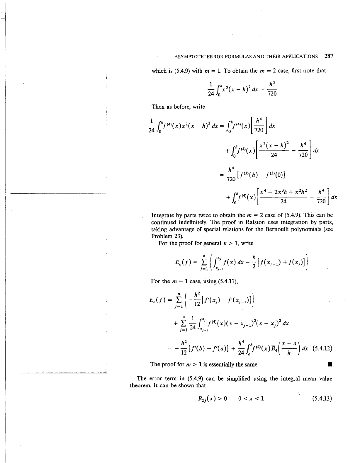
To obtain the m = 2 case, first note that
1
1h
2
h5
- x
2
(x-
h) dx = -
24 0 720
Then as before, write
Integrate by parts twice to obtain the
m = 2 case of (5.4.9). This can be
continued indefinitely. The proof in Ralston uses integration by parts,
taking advantage of special relations for the Bernoulli polynomials (see
Problem
23).
For the proof for general n >
1,
write
For
the m = 1 case, using (5.4.11),
h
2
h
4
Jb
_ ( x -
a)
=-
12
[/'(b)-
f'(a)]
+
24
aj<
4
>(x)B
4
-h-
dx (5.4.12)
The proof for m > 1
is
essentially the same.
•
The error term in (5.4.9) can be simplified using the integral mean value
theorem.
It
can be shown that
O<x<1
(5.4.13)
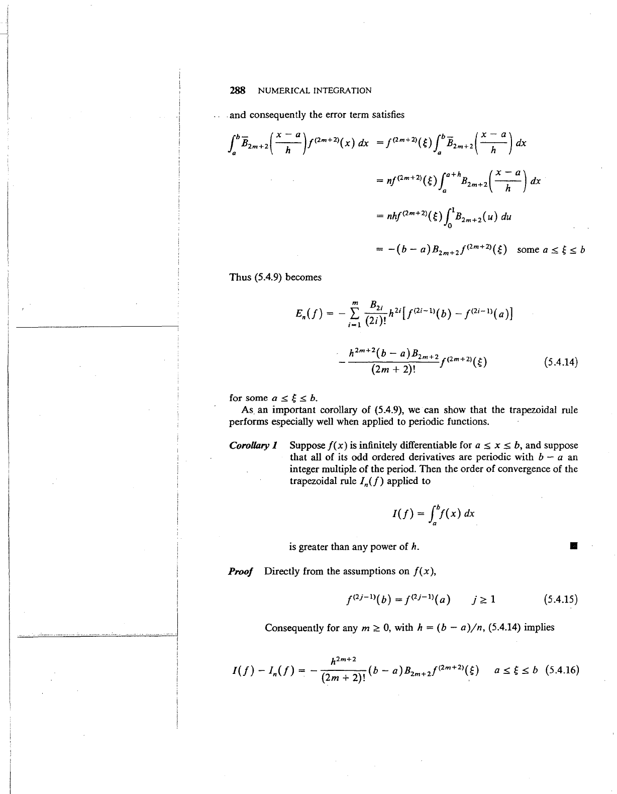
288 NUMERICAL INTEGRATION
.
and
consequently the error term satisfies
Thus
(5.4.9) becomes
· h
2
m+
2
(b -
a)B
-
2m+2
/(2m+2l(~)
(2m+
2)!
(5.4.14)
for some a
.::5:
~
.::5:
b.
As.
an
important
corollary
of
(5.4.9), we can show that the trapezoidal rule
performs especially well when applied to periodic functions.
Corollary I Suppose
f(x)
is infinitely differentiable for a
.::5:
x
.::5:
b, and suppose
that all
of
its
odd
ordered derivatives are periodic with b - a
an
integer multiple
of
the period. Then the order
of
convergence
of
the
trapezoidal rule
In(f)
applied to
is greater than
any
power
of
h.
•
Proof
Directly from the assumptions
on
f(x),
}~1
{5.4.15)
Consequently for any m
~
0, with h = (b -
a)jn,
(5.4.14) implies
h2m+2
I{!)-
In{!)=
-(
2
m+
2
)!
(b-
a)Bzm+zf<Zm+Z>(g)
a
.::5:
~
~
b (5.4.16)