Atkinson K. An Introduction to Numerical Analysis

ASYMPTOTIC ERROR FORMULAS

AND

THEIR APPLICATIONS

289

Thus

as

n ~

oo

(and h ~

0)

the rate of convergence

is

proportional to

h

2

m+

2

•

But m

was

arbitrary, which shows the desired result. •

This result is illustrated

in

Table 5.7 for

f(x)

= exp(cos(x)). The trapezoidal

rule is often the best numerical integration rule for smooth periodic integrands of

the type specified in the preceding corollary. For a comparison of the

Gauss-

Legendre formula and the trapezoidal rule for a one-parameter family of

periodic functions, of varying behavior,

see

Donaldson and Elliott (1972,

p.

592).

They suggest that the trapezoidal rule

is

superior, even for very peaked in-

tegrands. This conclusion improves on an earlier analysis that seemed

to

indicate

that Gaussian quadrature

was

superior for peaked integrands.

The Euler-MacLaurin summation fonnula Although it doesn't involve numeri-

cal integration, an important application of

(5.4.9)

or

(5.4.14)

is

to the summation

of

series.

Corollary 2 (Euler-MacLaurin summation formula) Assume

f(x)

is

2m

+ 2

times continuously differentiable for

0 5 x <

oo,

for some m

~

0.

Then for all n

~

1,

n n 1

L

f(J)

= 1

f(x)

dx

+

2[/(0)

+

f(n)]

j=O

. 0

m

B.

+ L

-;[!<2i-l>(n)

_ t<2i-l>(o)]

i=l

(2z

).

1

n_

- B (x)J<

2

m+

2

>(x)

dx

(2m +

2)!

0

2m+2

(5.4.17)

•

Proof

Merely substitute a =

0,

b = n into (5.4.9), and then rearrange the terms

appropriately.

•

Example

In

a later example

we

need the sum

00

1

s =I:

3/2

1 n

(5.4.18)

If

we

use the obvious choice

f(x)

=

(x

+

1)-

3

1

2

in (5.4.17), the results are

disappointing.

By

letting n

-+

oo,

we

obtain

1

oo

dx

1 m

B2·

s-

+ I (2i-l) 0

- o (x +

1)

3

/

2

2-

~

(2i)!/

( )

1

oo_

·

- 1 B (x)J<

2

m+

2

>(x)

dx

(2m

+

2)!

0

2m+2

•

••••••••

u

••

•

•••

)

290

NUMERICAL INTEGRATION

and the error term does not become small for any choice of m. But if

we

divide

the series

S into

two

parts,

we

are able to treat it very accurately.

Let

j(x)

=

(x

+

10)-

3

1

2

•

Then with m = 1,

oo 1

00

.

1

oo

dx 1

(1/6)

(-

l)

"

"/(

) + z + E

'f;;

n

312

=

~

1

= o (x + 10)

312

2(10)

312

-

-2-.

(10)

512

Since B

4

(x)

:2:

0,

j<

4

>(x) >

0,

we

have E <

0.

Also

1

00(

1 )

35

0 <

-E

< -1 -

j<

4

>(x) dx =

='=

1.08 X

10-

6

24

0

16

(1024)(10)

912

Thus

9

00

1

L

3/2

= .648662205 + E

10 n

By

directly summing

L(ljn

3

1

2

)

= 1.963713717,

we

obtain

00

1

L

3/2

= 2.6123759 + E 0 <

-E

< 1.08 X

10-

6

1 n

(5.4.19)

See Ralston (1965, pp. 134-138) for more information on summation techniques.

To appreciate the importance

of

the preceding summation method, it would have

been necessary to have added

3.43

X

10

12

terms in S to have obtained compara-

ble accuracy.

A generalized Euler-MacLaurin

formula

For integrals in which the integrand

is

not differentiable at some points, it

is

still often possible to obtain an asymptotic

error expansion. For the trapezoidal rule and other numerical integration rules

applied to integrands with algebraic

andjor

logarithmic singularities, see the

article Lyness and Ninham (1967). In the following paragraphs,

we

specialize

their results to the integral

a>O

(5.4.20)

with j E

cm+

1

[0,

1],

using the trapezoidal numerical integration rule.

Assuming

a is not an integer,

(5.4.21)

ASYMPTOTIC ERROR FORMULAS

AND

THEIR

APPLICATIONS

291

The term

0(1/nm+l)

denotes a quantity whose size is proportional to

1/nm+t,

or

possibly smaller. The constants are given by

2 r (a + j + 1) sin [ (

'1T

12)

(a

+

j)

H (a + j +

1)

.

= JU>(o)

cj

{2'1Tr+j+lj! .

d.=

0

J

for j even

2t(

"+

1)

d.=

(

-1)U-ll/

2

•

1

.

U>(1)

1·

odd

J

(2'1T);+l

g

with

g(x)

=

xaf(x),

f(x)

the gamma function,

and

t{p)

the zeta function,

00

1

t(

P)

=

L:

---:;

j=l}

p>1

(5.4.22)

For

0 < a < 1 with m = 1,

we

obtain the asymptotic error estimate

2f(

a+

1)

sin [( '1T/2)a]t( a +

i)/(0)

+

o(

n12)

En(!)=

(2'1T

t+lna+l

(5.4.23)

For

example with

I=

f5J(x)

dx,

and

using (5.4.19) for evaluating

t{f),

c =

t(t)

~

.208

4'1T

(5.4.24)

This is confirmed numerically in the example given

in

Table 5.6

in

Section 5.1.

For

logarithmic endpoint singularities, the results

of

Lyness

and

Ninham

(1967) imply

an

asymptotic error

f<;>rmula

(5.4.25)

for some p > 0 and some constant

c.

For

numerical purposes, this is essentially

0(1jnP).

To

justify this, calculate the following limit using L'Hospital's rule,

with p > q:

..

log(n)jnP

..

log(n)

Lmut = Lumt = 0

n--+oo

1/nq

n--+oo

np-q

This means that

log(n)jnP

decreases more rapidly

than

1/nq

for any q < p.

And

it

clearly decreases less rapidly than

1jnP,

although

not

by much.

-

....

:-.:..

--

···-

~.:·

..

____

; ....... :

-·

········-

·····-·-·-···-···

292

NUMERICAL INTEGRATION

For practical computation, (5.4.25)

is

essentially

0(1jnP).

For example,

calculate the limit of successive errors:

I-1

Limit n

n-+oo

I-

/

2

n

. . c

·log(n)jnP

log(n}

Lnrut

= Limit2P ·

---

n-+oo

c

·log(2n)j2PnP

n-+oo

log(2n}

1

= Limit2P. =

2P

n-+oo

1+(log2jlogn)

This

is

the same limiting ratio

as

would occur if the error were just O(lfn.P).

Aitken extrapolation Motivated by the preceding,

we

assume that the integra-

tion formula has an asymptotic error formula

c

I-I=-

n

nP

p>O

{5.4.26)

This

is

not always valid. For example, Gaussian quadrature does not usually

satisfy (5.4.26), and the trapezoidal rule applied to periodic integrands does not

satisfy it. Nonetheless, many numerical integration rules do satisfy it, for a wide

variety of integrands.

Using this assumed form for the error,

we

attempt to

estimate the error. An analogue of this work

is

that on Aitken extrapolation in

Section 2.6.

First

we

estimate p. Using (5.4.26),

(I

- In) -

(I

- I 2n)

(I-

/2n) -

(I-

/4,)

This gives a simple

way

of computing p.

(5.4.27)

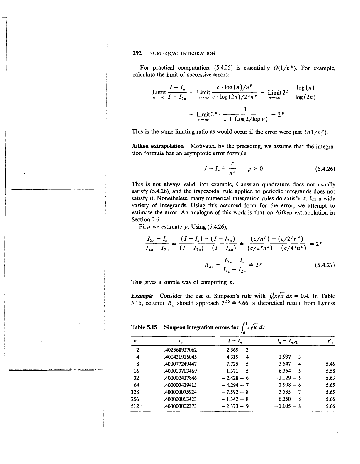
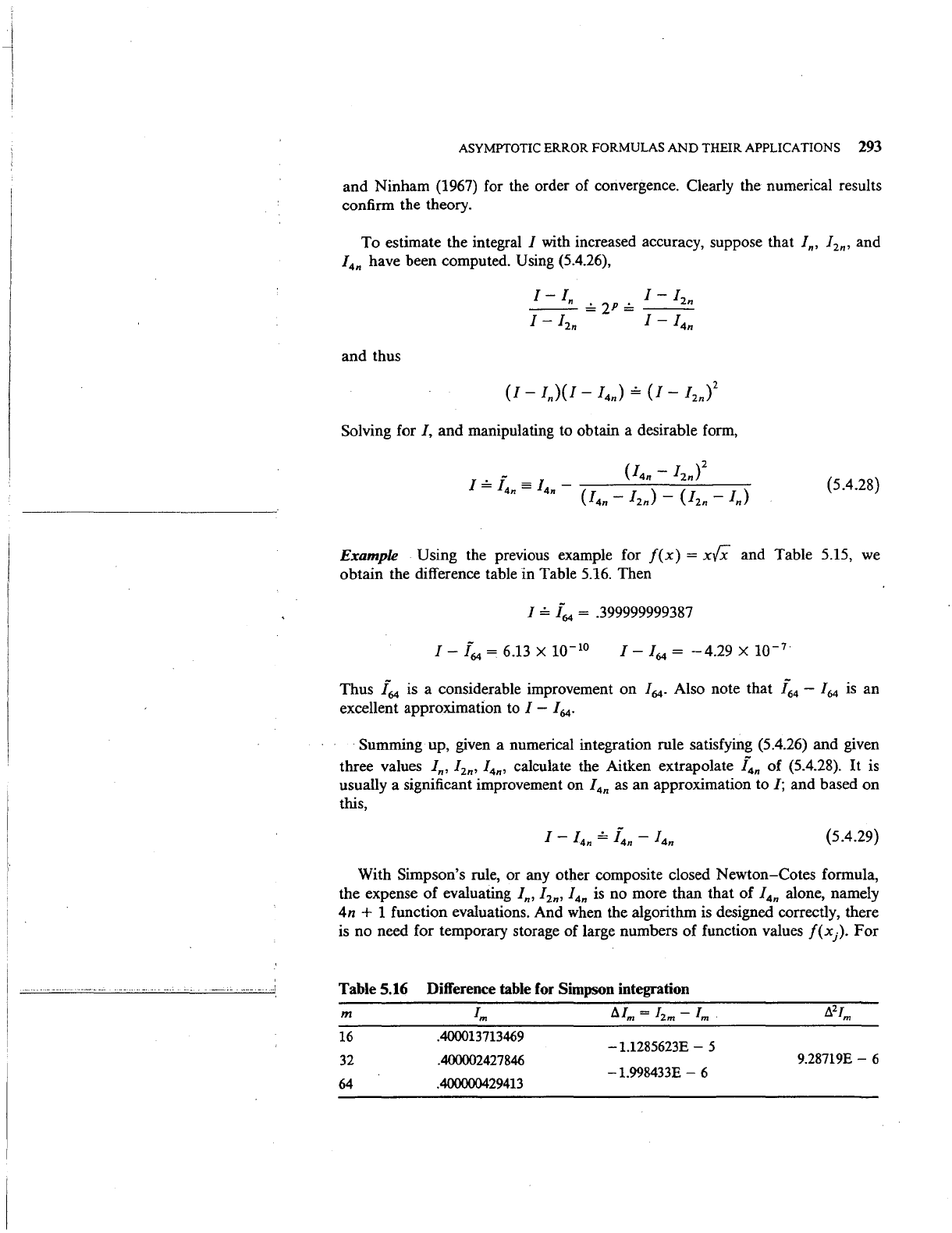
Example Consider the

use

of Simpson's rule with

/Jx/X

dx = 0.4. In Table

5.15, column Rn should approach

2

·

5

= 5.66, a theoretical result from Lyness

Table 5.15

Simpson integration errors for

1

xiX

dx

0

n

In

I-

I,

I,-

In/2

Rn

2 .402368927062

-2.369-

3

4

.400431916045

-4.319-

4

-1.937-

3

8

.400077249447

-7.725-

5

-3.547-

4

5.46

16

.400013713469

-1.371-

5

-6.354-

5

5.58

32 .400002427846

-2.428-

6

-1.129-

5

5.63

64 .400000429413

-4.294-

7

-1.998-

6

5.65

128

.400000075924

-7.592-8

-3.535-

7

5.65

256 .400000013423

-1.342-

8

-6.250-

8

5.66

512 .4000000023

73

-2.373-

9

-1.105-

8

5.66

..

1

ASYMPTOTIC ERROR FORMULAS

AND

THEIR APPLICATIONS

293

and Ninham (1967) for the order of convergence. Clearly the numerical results

confirm the theory.

To estimate the integral

I with increased accuracy, suppose that In, I

2

n,

and

I

4

n have been computed. Using (5.4.26),

and thus

Solving for

I,

and manipulating to obtain a desirable form,

(5.4.28)

Example Using the previous example for

f(x)

=

xVx

and Table 5.15,

we

obtain the difference table in Table

5.16.

Then

I = i

64

= .399999999387

I-

f

64

=

6.13

X

10-

10

I-

I

64

=

-4.29

X

10-

7

Thus [

64

is a considerable improvement on I

64

•

Also note that

I:

4

- I

64

is

an

excellent approximation

to

I-

I

64

•

Summing up, given a numerical integration rule satisfying (5.4.26) and given

three values

In, I

2

n,

I

4

n,

calculate the Aitken extrapolate

~n

of (5.4.28).

It

is

usually a significant improvement on

I

4

n

as

an approximation to

I;

and based on

this,

(5.4.29)

With Simpson's rule, or any other composite closed Newton-Cotes formula,

the expense of evaluating

In, I

2

n,

I

4

n is no more than that of I

4

n alone, namely

4n

+ 1 function evaluations. And when the algorithm is designed correctly, there

is no need for temporary storage of large numbers of function values

f(x).

For

Table 5.16 Difference table for Simpson integration

m

/m

fl[m

=

[2m-

Jm

·

fl2Jm

16

.400013713469

-1.1285623E -

5

32 .400002427846

9.28719E-

6

64

.400000429413

-1.998433E - 6

294 NUMERICAL INTEGRATION

that

reason,

one

should never use Simpson's rule with

just

one value of the index

n.

With

no

extra expenditure

of

time, and with only a slightly more complicated

algorithm,

an

Aitken extrapolate and an error estimate can be produced.

Richardson

extrapolation

If

we

assume sufficient smoothness for the integrand

f(x)

in

our

integral

I(f),

then

we

can write the trapezoidal error

term

(5.4.9) as

.

d(O)

I-I

=-

2

-+-

4

-+···+~+F

n

n2

n4

n2m

n.m

(5.4.30)

where

In

denotes the trapezoidal rule, and

(

)

2m+2

b-a

h-

(x-a)

Fn,m

= (

2

m+

2

)!n2m+2l

B2m+2

-h-

J<Zm+Z>(x)

dx

(5.4.31)

Although the series dealt with are always finite and have an error term, we will

usually

not

directly concern ourselves with it.

.For

n even, ·

4d(O)

16d(O)

64d(O)

I-I

=-2-+

__

4_+

__

6_+···

n/2

n1 n4 n6

Multiply (5.4.30)

by

4

and

subtract from

it

(5.4.32):

-12d(O)

6Qd(O)

4( I - I ) -

(I

- I ) =

4

- -

6

- -

• • •

n

n/2

n4

n6

Define

1

I(l)

= _

[4I(0)

_

I(O)

]

n 3 n

n/1

2Qd(O)

6

~-···

n even n:::::2

and

/~

0

>

= Im.

We

call {

/~

1

>}

the Richardson extrapolate

of

{

/~

0

>

}.

The

sequence

/

(1) .

J(l)

2 ' 4 ' 6 '

•••

is a new numerical integration rule.

For

the error,

d(l)

I -

J<l>

=

_4_

+

_6_

+

n

n4

n6

d

(l)

=

-4d(O)

d(l)

=

-2Qd(O)

4 4 ' 6 6 '

•••

(5.4.32)

(5.4.33)

(5.4.34)

(5.4.35)

.i

ASYMPTOTIC ERROR FORMULAS AND

THEIR

APPLICATIONS 295

To

see the explicit formula for

I~

1

>,

let h =

(b-

a)jn

and x

1

=a+

jh for

j =

0,

1,

...

, n. Then using (5.4.33) and the definition of the trapezoidal rule,

4h [ 1 1 ]

I(l) = - - { + f + f + f +

...

+/,

+

-/,

n

3

2

JO

l 2 3 n-1

2

n

h .

IP)

= J[/o +

4/l

+ 2/2 +

4/3

+ · · ·

+2fn-2

+ 4/n-1 +

fn]

(5.4.36)

which

is

Simpson's rule with n subdivisions.

For

the error, using (5.4.35) and

(5.4.31),.

h4 h6

I_

I(1J = _

-[J(3l(b)

_ J(3l(a)] +

---(J<5l(b)

_

J<S>(a)]

+

...

n

180

1512

(5.4.37)

This means that the work on the Euler-MacLaurin formula transfers to Simpson's

rule by means of some simple algebraic manipulations. We omit any numerical

examples since they would just be Simpson's rule, due to (5.4.36).

The

preceding argument, which led to

I~

1

>,

can

be

continued to produce other

new formulas.

As

before, if n is a multiple

of

4,

then

16d(l)

64d(

1

)

I-

I

=

__

4_

+

__

6_

+

...

n/2

n4

n6

.

-48d(

1

)

16(I-

I<

1

>)-

(I-

I<

1

>)

=

6

+ · · ·

n

n/2

n6

I=

16J(l) - J(l) 48d(l) .

n

n/2

___

6_

+

...

15

15n

6

(5.4.38)

Then

d(2)

(

2)

6 8

[-[

=-+-+···

n

n6

n8

(5.4.39)

with

16I(1) - J(l)

J(2)

= n

n/2

n

15

n~4

(5.4.40)

and

n divisible by

4.

We call

{1~

2

>}

the Richardson extrapolate of

{1~

1

>

}.

If

we

derive the actual integration weights

of

Jp>,

in analogy with (5.4.36),

we

will find

that

Jp>

is simply the composite Boole's rule.

296

NUMERICAL INTEGRATION

Using the preceding formulas,

we

can obtain useful estimates of the error.

Using (5.4.39),

16I(l) - I(l)

d(2)

I - IP) = n

nj2

- I(l) +

_6_

+ • . •

15

" n

6

I(l) - I(l)

d(2)

n

n/2

+

_6_

+

...

15

n

6

Using h =

(b-

a)jn,

1

I_

I

=

-(I

_

I]

+

O(h6)

n

15

n

n/2

(5.4.41)

and thus

1

I_

I<Il

~

_

(I

_

I

]

n

15

n

n/2

(5.4.42)

since both terms are

O(h

4

)

and the remainder term

is

O(h

6

).

This

is

called

Richardson's error estimate for Simpson's rule.

This extrapolation process can be continued inductively. Define

4ki(k-1)-

J(k-1)

I(k)

= n

nj2

n

4k-

1

(5.4.43)

with

n a multiple of

2k,

k

~

1.

It

can be shown that the error has the form

d(k)

(

k)

2k+2

I-I

=--+···

n

n2k+2

(5.4.44)

with Ak a constant independent

off

and

h,

and

Finally, it can

be

shown that for any f E

C[a,

b],

Limitl~k>(J)

=I(!)

(5.4.45)

n-+oo

The rules

I~k>(J)

for k > 2 bear no direct relation to the composite

Newton-Cotes rules. See Bauer et

al.

(1963) for complete details.

Romberg

integration Define

k =

0,1,2,

...

(5.4.46)

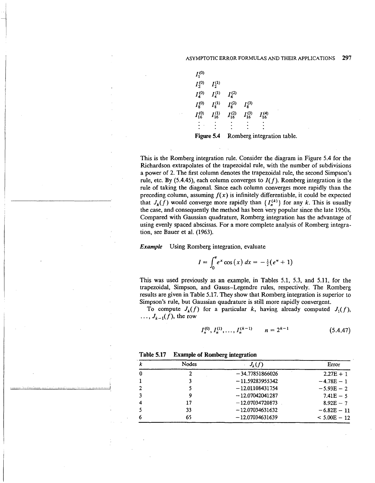
ASYMPTOTIC ERROR FORMULAS AND

THEIR

APPLICATIONS 297

J(O)

I

f(O)

2

J(1)

2

J(O)

4

Jjl>

/(2)

4

J(O)

8

J(1)

8

/(2)

8

J(3)

8

f(O)

16

J(1)

16

/(2)

16

J(3)

16

J(4)

16

Figure

5.4

Romberg integration table.

This is the Romberg integration rule. Consider the diagram in Figure 5.4 for the

Richardson extrapolates of the trapezoidal rule, with the number of subdivisions

a power of

2.

The first column denotes the trapezoidal rule, the second Simpson's

rule, etc.

By

(5.4.45), each column converges to

/(f).

Romberg integration

is

the

rule

of

taking the diagonal. Since each column converges more rapidly than the

preceding column, assuming

f(x)

is

infinitely differentiable, it could be expected

that

Jk(f)

would converge more rapidly than

{I~kl}

for any k. This

is

usually

the case, and consequently the method has been

very popular since the late 1950s.

Compared with Gaussian quadrature, Romberg integration has the advantage of

using evenly spaced abscissas. For a more complete analysis of Romberg integra-

tion, see Bauer et al. (1963).

Example Using Romberg integration, evaluate

This

was

used previously

as

an example, in Tables 5.1,

5.3,

and 5.11, for the

trapezoidal, Simpson, and Gauss-Legendre rules, respectively. The Romberg

results are given in Table

5.17.

They show that Romberg integration

is

superior to

Simpson's rule,

but

Gaussian quadrature

is

still more rapidly convergent.

To compute

Jk(f)

for a particular k, having already computed J

1

(f),

...

, Jk_

1

(f),

the row

Table 5.17 Example of Romberg integration

k Nodes

Jk

(/)

0

1

2

3

4

5

6

2

3

5

9

17

33

6S

-34.77851866026

-11.59283955342

-12.01108431754

-12.07042041287

-12.07034720873

-12.07034631632

-12.07034631639

{5.4.47)

Error

2.27E + 1

-4.78E-

1

-5.93E-

2

7.41E-

5

8.92E-

7

-6.82E-

11

<

5.00E-

12

298 NUMERICAL INTEGRATION

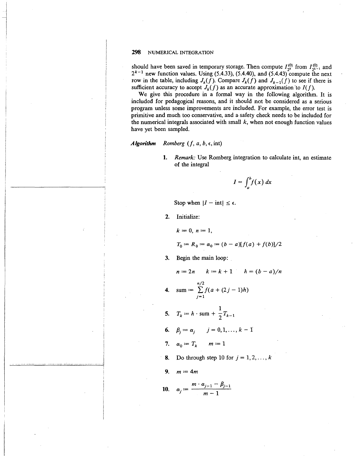
should have been saved in temporary storage. Then

compute/~~)

from

Ii?~~

and

2k-

1

new function values. Using (5.4.33), (5.4.40), and (5.4.43) compute the next

row in the table, including

Jk(f).

Compare

Jk(f)

and Jk_

1

(f)

to see if there

is

sufficient accuracy to accept

Jk(f)

as

an accurate approximation ·to

/(/).

We give this procedure

in

a formal way in the following algorithm. It

is

included for pedagogical reasons, and it should

not

be considered

as

a serious

program unless some improvements are included.

For

example, the error test is

primitive and much too conservative, and

a·

safety check needs to be included for

the numerical integrals associated with small

k, when not enough function values

have yet been sampled.

Algorithm Romberg

(f,

a, b,

£,

int)

1.

Remark: Use Romberg integration to calculate int, an estimate

of the integral

Stop when

I/-

inti

~

£.

2.

Initialize:

k

:=

0, n

:=

1,

T

0

:= R

0

:= a

0

:=

(b-

a)[f(a)

+

/(b)]/2

3. Begin the main loop:

n

:=

2n

k

:=

k + 1

h

=

(b-

a)jn

n/2

4.

sum:=

L

f(a

+

(2}-

1)h)

j=1

1

5.

Tk

:= h

·sum+

2Tk_

1

6.

f3j

:=

aj

j = 0, 1,

...

, k - l

8.

Do

through step

10

for j = 1, 2,

...

, k

9. m

:=

4m

10.

m.

aj-1-

f3j-1

aj

:=

m-

1

Atkinson K. An Introduction to Numerical Analysis

Подождите немного. Документ загружается.