Atkinson K. An Introduction to Numerical Analysis
Подождите немного. Документ загружается.

EULER'S METHOD
341
There are special numerical methods for m th order equations,
but
these have
been developed to a significant extent only for m =
2,
which arises in applica-
tions
of
Newtonian mechanics from Newton's second law
of
mechanics. Most
high-order equations are solved by first converti,...g them to
an
equivalt:nt first-
order
system, as was just described.
6.2
Euler's
Method
The
most popular numerical methods for solving (6.0.1) are called finite
difference methods.
Approximate values are obtained for the solution
at
a
set
of
grid points
(6.2.1)
and the approximate value at each X
1
,
is
obtained by using some
of
the
values
obtained
in
previous steps.
We
begin with a simple
but
computationally ineffi-
cient
method
attributed to Leonhard Euler.
The
analysis
of
it has many
of
the
features
of
the
analyses
of
the more efficient finite difference methods, but
without
their
additional complexity. First we give several derivations
of
Euler's
method,
and
follow with a complete convergence
and
stability analysis for it. We
give
an
asymptotic
error
formula,
and
conclude
the
section by generalizing the
earlier results to systems
of
equations.
As before,
Y(x)
will denote the true solution
to
(6.0.1):
Y'(x)
=
f(x,
Y(x))
(6.2.2)
The
approximate solution will
be
denoted by
y(x),
and
the values
y(x
0
),
y(x
1
),
•••
,
y(xn),
...
will often be denoted by y
0
,
y
1
,.
••
,
y,,
....
An
equal grid
size h > 0
will
be
used to define the node points,
j
=0,1,
...
When
we
are
comparing numerical solutions for various values
of
h, we will also
use the notation y
11
(x)
to·refer to
y(x)
with stepsize h. The problem (6.0.1) will
be
solved
on
a fixed finite interval, which will always
be
denoted by
[x
0
,
b]. The
notation
N(h)
will denote the largest index N for which
In
later sections, we discuss varying the stepsize
at
each xn, in order to control
the
error. ·
Derivation
of
Euler's
method
Euler's method
is
defined by
Yn+l
= Y, +
hf(xn,
Yn)
n = 0,
1,2,
...
(6.2.3)
wit!t
Yo
= Y
0
•
Four_
viewpoints
of
it are given.
I
I
_
_I
342
NUMERICAL
METHODS FOR ORDINARY
DIFFERENTIAL
EQUATIONS
z =
Y(x)
--+---~--------~---------x
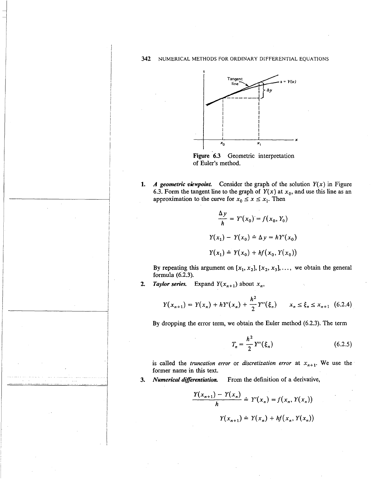
Figure
6.3
Geometric interpretation
of Euler's method.
1.
A geometric viewpoint. Consider the graph of the solution
Y(x)
in Figure
6.3.
Form
the tangent line to the graph
of
Y(x)
at
x
0
,
and
use this line as an
approximation to the curve for
x
0
::;
x::;
x
1
•
Then
Y(x
1
)-
Y(x
0
)
=
!J..y
=
hY'(x
0
)
Y(x
1
)
=
Y(x
0
)
+
hf(x
0
,
Y(x
0
))
By repeating this argument on
[x
1
,
x
2
],
[x
2
,
x
3
],
•••
, we obtain the general
formula (6.2.3).
2.
Taylor series. Expand Y(xn+l) about xn,
By dropping the error term,
we
obtain the Euler method (6.2.3). The term
h2
T
=-
Y"(~
)
n 2 n
(6.2.5)
is
called the truncation error or discretization error
at
xn+I·
We
use
the·
former name in this text.
3.
Numerical differentiation. From the definition of a derivative,
Y(x
) -
Y(x
)
n+l n =
Y'(xn)
=
f(xn,
Y(xJ)
h
EULER'S METHOD
343
a
a+h
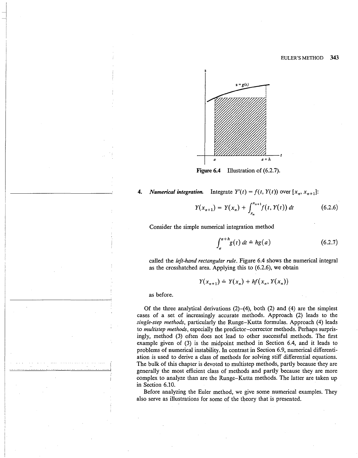
Figure
6.4 Illustration of (6.2.7).
4.
Numerical integration. Integrate Y'(t) =
f(t,
Y(t))
over [xn, xn+d:
Y(xn+l) =
Y(xn)
+
Jxn+tf(t,
Y(t))
dt
x.
(6.2.6)
Consider the simple numerical integration method
Ja+hg(t)
dt,;,
hg(a)
a
(6.2.7)
called the left-hand rectangular rule. Figure 6.4 shows the numerical integral
as the crosshatched area. Applying this to
(6.2.6),
we
obtain
as before.
Of
the three analytical derivations (2)-(4), both (2) and (4) are the simplest
cases of a set of increasingly accurate methods. Approach
(2)
leads to the
single-step methods, particularly the
Runge-Kutta
formulas. Approach
(4)
leads
to
multistep methods, especially the predictor-corrector methods. Perhaps surpris-
ingly, method
(3)
often does not lead to other successful methods. The first
example given of
(3)
is
the midpoint method
in
Section 6.4, and it leads to
problems
of
numerical instability. In contrast in Section 6.9, numerical differenti-
ation is used to derive a class of methods for solving stiff differential equations.
The bulk of this chapter
is
devoted to multistep methods, partly because they are
generally the most efficient class of methods
and
partly because they are more
complex to analyze than are the Runge-Kutta methods. The latter are taken up
in Section
6.10.
Before analyzing the Euler method,
we
give some numerical examples. They
also serve as illustrations for some of the theory that is presented.
!
!
J
344
NUMERICAL METHODS FOR ORDINARY DIFFERENTIAL EQUATIONS
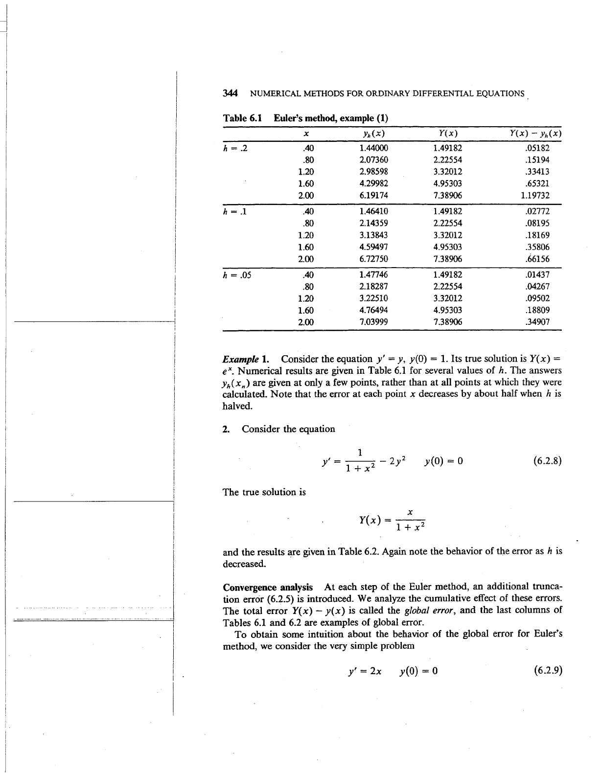
Table
6.1
Euler's method, example
(1)
X
Yh(x)
Y(x)
Y(x)
- Yh(x)
h = .2 .40
1.44000 1.49182 .05182
.80
2.07360
2.22554 .15194
1.20 2.98598 3.32012
.33413
1.60
4.29982 4.95303 .65321
2.00
6.19174
7.38906 1.19732
h
= .1
.40
1.46410 1.49182 .02772
.80
2.14359
2.22554
.08195
1.20
3.13843 3.32012 .18169
1.60
4.59497
4.95303 .35806
2.00
6.72750 7.38906
.66156
h
= .05 .40
1.47746 1.49182 .01437
.80
2.18287 2.22554 .04267
1.20
3.22510
3.32012
.09502
1.60
4.76494 4.95303 .18809
2.00
7.03999 7.38906 .34907
Example
1.
Consider the equation
y'
=
y,
y(O) = 1. Its true solution
is
Y(x)
=
ex. Numerical results are given in Table
6.1
for several values of
h.
The answers
yh(xn)
are given
at
only a
few
points, rather than
at
all points at which they were
calculated. Note that the error
at
each point x decreases by about half when h
is
halved.
2.
Consider the equation
The true solution
is
y(O)
= 0
X
Y(x)
=
--
1 + x
2
(6.2.8)
and the results
a,re
given in Table 6.2. Again note the behavior of the error as h
is
decreased.
Convergence analysis
At
each step of the Euler method, an additional trunca-
tion
error (6.2.5) is introduced. We analyze the cumulative effect of these errors.
The total error
Y(x) -
y(x)
is
called the global
error,
and
the last columns of
Tables
6.1
and
6.2 are examples of global error.
To
obtain some intuition about the behavior of the global error for Euler's
method, we consider the very simple problem
y'
=
2x
y(O) = 0
(6.2.9)
···r
·I
-·
. -
--~--
·-
-
.....
---
-
..
-
--
....
- .......... i
EULER'S METHOD
345
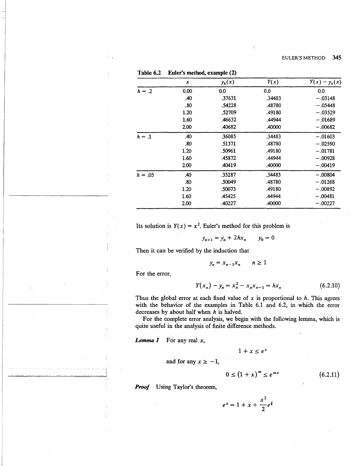
Table 6.2
Euler's method, example (2)
X
Yh(x)
Y(x)
Y(x)
-
Yh(x)
h =
.2
0.00 0.0
0.0
0.0
.40
.37631 .34483
-.03148
.80
.54228
.48780
-.05448
1.20 .52709 .49180
-.03529
1.60
.46632 .44944
-.01689
2.00
.40682
.40000
-.00682
h =
.1
.40
.36085
.34483
-.01603
.80
.51371
.48780
-.02590
1.20
.50961
.49180
-.01781
1.60
.45872
.44944
-.00928
2.00
.40419
.40000
-.00419
h =
.05
.40
.35287
.34483
-.00804
.80
.50049 .48780
-.01268
1.20
.50073 .49180
-.00892
1.60
.45425 .44944
-.00481
2.00
.40227 .40000
-.00227
Its
solution is
Y(x)
= x
2
•
Euler's
method
for this problem is
Yn+l
=
Yn
+ 2hxn
Yo=
0
Then
it
can
be
verified
by
the induction
that
For
the
error,
(6.2.10)
Thus
the
global error
at
each fixed value
of
x is proportional to h. This agrees
with
the
behavior
of
the examples
in
Table 6.1
and
6.2, in which the error
decreases
by
about
half when h is halved.
For
the
complete error analysis, we begin with the following lemma, which is
quite useful
in
the analysis
of
finite difference methods.
Lemma I
For
any real x,
and
for any x
::?:
- 1,
(6.2.11)
Proof
Using Taylor's theorem,
I
I
--
I
I
346 NUMERICAL METHODS FOR ORDINARY DIFFERENTIAL EQUATIONS
with g between 0 and x. Since the remainder is always positive, the first
result
is
proved. Formula (6.2.11) follows easily. •
For
the
remainder of this chapter, it is assumed that the function
f(x,
y)
satisfies
the
following stronger Lipschitz condition:
-
oo
<
Y1,
Y2
<
oo
( 6.2.12)
for some K
~
0. Although stronger than necessary, it will simplify the proofs.
And
given a function
f(x,
y)
satisfying
the
weaker condition (6.1.1)
and
a
solution Y(x) to the initial value problem (6.0.1), the function f can be modified
to satisfy (6.2.12) without changing the solution Y(x)
or
the essential character
of
the problem (6.0.1) and its numerical solution. [See Shampine
and
Gordon
(1975), p. 24, for the details].
Theorem 6.3 Assume that the solution
Y(x)
of
(6.0.1) has a bounded second
derivative on
[x
0
,
b]. Then the solution
{h(xn)lx
0
:s;
xn
_:s;
b}
obtained
by
Euler's method (6.2.3) satisfies
where
and
e
0
= Y
0
- Yh(xo)·
If
in addition,
[
e(b-x
0
)K
_
1]
+ K -r(h) (6.2.13)
(6.2.14)
ash~
0
(6.2.15)
for some c
1
~
0 (e.g., if Y
0
= y
0
for all h), then there is a constant
B
~
0 for which
Max
IY{xn)-
Yh(xn)
I.:$;
Bh
x
0
s;x.
s;
b
{6.2.16)
Proof Let
en=
Y(xn)
-
y(xn),
n
~
0, and recall the definition
of
N(h)
from
the beginning
of
the section. Define
0
_:s;
n
_:s;
N(h)
-1
·i
..........
·--
~I
EULER'S METHOD
347
based on the truncation error in (6.2.5). Easily
using (6.2.14). From (6.2.4), (6.2.2), and (6.2.3), we have
Yn+l
=
Yn
+
hj(xn,
yJ
0.:;;:
n.:;;:
N(h)-
1
(6.2.17)
(6.2.18)
We are using the common notation
Yn
= Y(xn). Subtracting (6.2.18) ·
from (6.2.17),
(6.2.19)
and taking bounds, using (6.2.12),
!en+ll
,:;;:
len!
+
hK!
Yn-
Ynl
+
hi'Tnl
len+d
.:;;:
(1
+ hK)!enj + h'T(h)
·o.:;;:
n.:;;:
N(h)-
1 (6.2.20)
Apply (6.2.20) recursively to obtain
Using the formula for the sum
of
a finite geometric series,
rn-
1
1 + r + r
2
+ · · ·
+rn-l
=
--
r
=F
1
r-1
(6.2.21)
we obtain
n
[(1
+
hKr-
1]
len!
.:;;:
(1
+
hK)
je
0
! + K 'T(h)
(6.2.22)
Using Lemma
1,
and this with (6.2.22) implies the main result (6.2.13).
The remaining result (6.2.16) is a trivial corollary
of
(6.2.13) with the
constant
B given by
B = c
e<b-xo)K
+ .
--""
[
e(b-xo)K-
1]
IIY"II
1
K 2
This completes the proof.
•
i
I
I
I
I
·-
---
--
...
. .
...
...
........
--
__
I
348 NUMERICAL METHODS FOR ORDINARY DIFFERENTIAL EQUATIONS
· The result (6.2.16) implies
that
the error should decrease by at least one-half
when the stepsize
h
is
halved. This
is
confirmed
in
the examples of Table
6.1
and
6.2.
It
is
shown later in the section that (6.2.16)
gives
exactly the correct rate of
,convergence (also
see
Problem 7).
The bound
(6.~.16)
gives
the correct speed
of
convergence for Euler's method,
but
the multipl)'ing constant B
is
much too large for most equations. For
example, with the earlier example
(6.2.8), the formula (6.2.13)
will
predict that
the bound grows with
b. But clearly from Table 6.2, the error decreases with
increasing
x.
We
give
the following improvement of (6.2.13)
to
handle many
cases such as (
6.2.8).
Corolkuy Assume the same hypotheses
as
in Theorem 6.3; in addition, assume
that
aJ(x,
y)
ay
~
o
( 6.2.23}
for x
0
~
x
~
b,
-
oo
< y <
oo.
Then for all sufficiently small
h,
•
Proof
Apply the mean value theorem to the error equation (6.2.19):
(6.2.25)
with
t,.
between
Yh(x,.)
and Y(x,.). From the convergence of
Yh(x)
to
Y(x) on
[x
0
,.b],
we
know that the partial derivatives
aj(xn,
tn)/ay
approach
aj(x,
Y(x))jay,
and thus they must be bounded in magnitude
over
[x
0
,
b).
Pick h
0
> 0 so that
( 6.2.26)
for all h
~
h
0
.
From (6.2.23),
we
know the left side
is
also bounded
above by
1,
for all h. Apply these results
to
(6.2.25) to get
h2
len+ll
~
lenl
+
2IY"a,.)
I
( 6.2.27}
By
induction,
we
can show
h2
le,.l
~
leol
+
T[IY"(~o)l
+ · · · + IY"an-1)1]
which easily leads to
(6~2.24).
•
_
...
l
EULER'S METHOD 349
Result (6.2.24)
is
a considerable improvement over the earlier bound (6.2.13);
the exponential
exp(K(b-
x
0
))
is replaced by
b-
x
0
(bounding
x,-
x
0
),
which increases less rapidly with
b.
The theorem does not apply directly to the
earlier example
(6.2.8), but a careful .examination of the proof in this case
will
show that the proof
is
still valid.
Stability analysis Recall the stability analysis for the initial value problem,
given in Theorem
6.2. To consider a similar idea for Euler's method,
we
consider
the numerical method
z,+
1
=
z,
+
h[f(x,,
zJ
+ S{x,)]
0
~
n
~
N(h)-
1 (6.2.28)
with z
0
= y
0
+
c.
This
is
in analogue to the comparison
of
(6.1.5) with (6.0.1),
showing the stability of the initial value problem.
We
compare the two numerical
solutions
{z,}
and {Y,}
ash~
0.
Let
e,
=
z,-
y,,
n;;:::
0.
Then e
0
=
c,
and subtracting (6.2.3) from (6.2.28),
e,+
1
= e, +
h[f(x,,
z,)-
f(x,,
y,)] +
h8(x,)
This has exactly the same form
as
(6.2.19). Using the same procedure as that
following
(6.2.19),
we
have
Consequently, there are constants k
1
,
k
2
,
independent of h, with
{6.2.29)
This is the analogue
to
the result (6.1.4) for the original problem (6.0.1). This says
that Euler's method
is
a stable numerical method for the solution of the initial
value problem
(6.0.1).
We
insist that
all
numerical methods for initial value
problems possess this form of stability, imitating the stability
of
the original
problem
(6.0.1). In addition,
we
require other forms of stability
as
well, which are
introduced later. In the future
we
take S(x) = 0 and consider only the effect of
perturbing the initial value
Y
0
•
This simplifies the analysis, and the results are
equally useful.
Rounding
error
analysis Introduce an error into each step of the Euler method,
with each error derived from the rounding errors of the operations being
performed. This number, denoted by
p,, is called the local rounding error. Calling
the resultant numerical values·
j,,
we
have
Yn+l
=
Yn
+
hf(x,.,
Y,.)
+
Pn
n =
0,1,
...
,
N(h)
-1
{6.2.30)
The values
Y,
are the finite-place numbers actually obtained in the computer, and
y,
is the value that would be obtained if exact arithmetic were being used. Let
l
I
I
..
..
. .
........
·--··
·-
.
····-·
.........
j
i
I
I
I
i
I
I
; .
350
• NUMERICAL METHODS FOR ORDINARY DIFFERENTIAL EQUATIONS
· p
(h)
be a bound on the rounding errors,
p(h)
=
Max
IPnl
OsnsN(h)-1
(6.2.31)
In
a practical situation, using a
fixed
word length computer, the bound
p(h)
does
not decrease
as
h -
0.
Instead, it remains approximately constant, and
p(h)/IIYIIoo will be proportional to the unit roundoff u on the computer, that is,
the smallest number
u for which 1 + u > 1
[see
(1.2.12) in Chapter
1].
To
see the effect of the roundoff errors in (6.2.30), subtract
it
from the true
solution in
(6.2.4), to obtain
where
e,.
=
Y(xn)
-
j,.
Proceed
as
in the proof of Theorem
6.3,
but identify
-r,.
- p,./h with
-r,.
in the earlier proof. Then
we
obtain
(6.2.32)
To
further examine this bound, let p(h)/IIYIIoo
,;,
u,
as
previously discussed.
Further assume that
Y
0
= y
0
•
Then
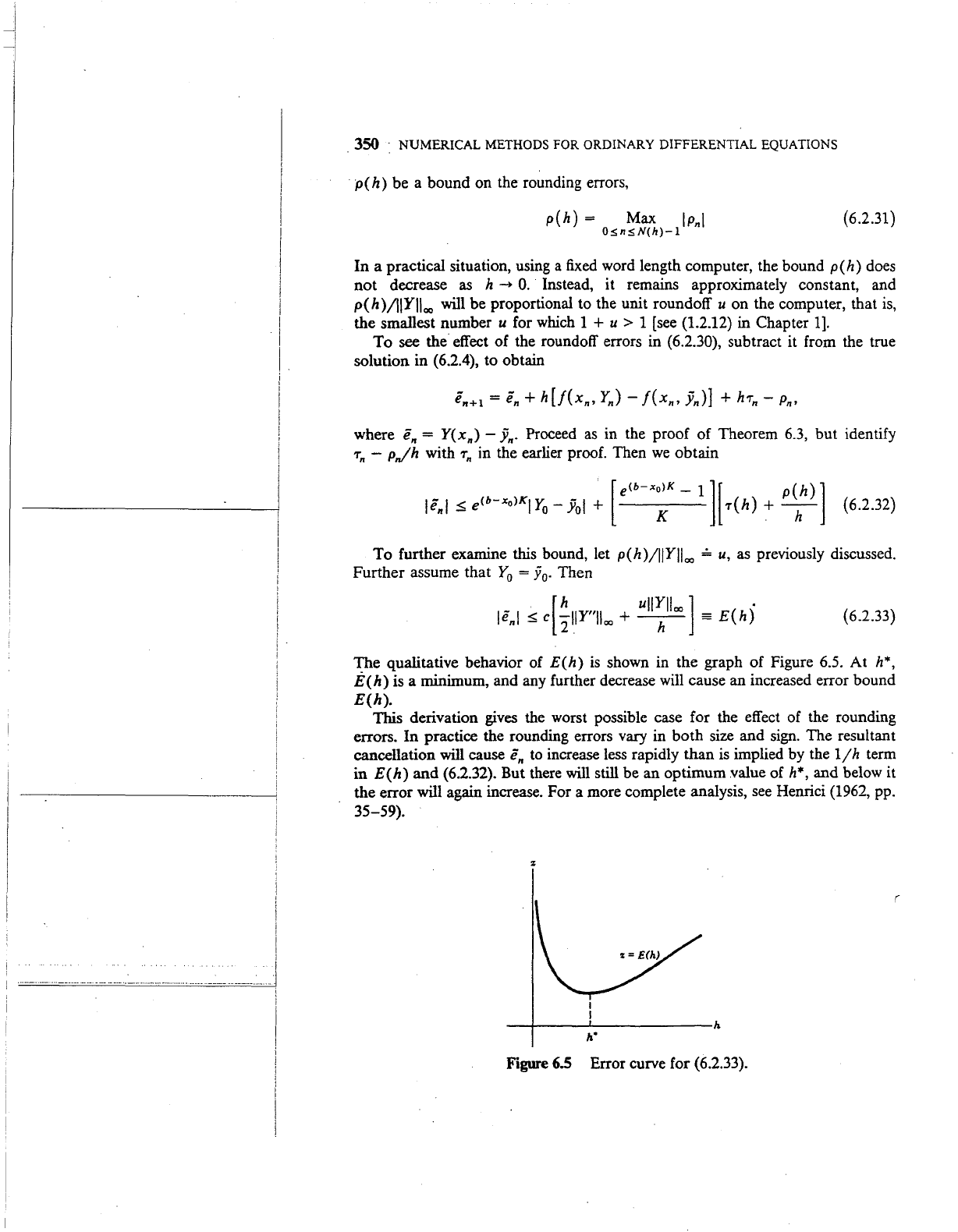
(6.2.33)
The qualitative behavior of
E(h)
is
shown in the graph of Figure 6.5. At h*,
E
(h)
is a minimum, and any further decrease will cause an increased error bound
E(h).
This derivation gives the worst possible case for the effect of the rounding
errors. In practice the rounding errors vary in both size and sign. The resultant
cancellation will cause
e,
to
increase less rapidly than
is
implied by the
ljh
term
in
E(h)
and (6.2.32). But there will still be an optimum value of h*, and below it
the error will again increase. For a more complete analysis,
see
Henrici (1962, pp.
35-59).
(
__
,_
____
~------------h
h"
Figure
6.5 Error curve for (6.2.33).