Banner A. The Calculus Lifesaver: All the Tools You Need to Excel at Calculus
Подождите немного. Документ загружается.


266 • Sketching Graphs
So you can see that the curve looks roughly like y = x
2
with some strange
stuff going on near x = 0, but you can’t really make out the details. This
really illustrates the difference between “plotting” and “sketching” a graph.
After all, the graphing calculator has just plotted enough points to make the
curve look smooth, but it doesn’t emphasize the interesting features of the
graph. You might get a better idea if you zoom in, but then you wouldn’t see
the behavior for large x. Even though it’s inaccurate, our rough sketch above
is much more useful for understanding what’s really going on, especially as
far as turning points and points of inflection are concerned: it shows exactly
where all these features are.
C h a p t e r 13
Optimization and Linearization
We’re now going to look at two practical applications of calculus: optimiza-
tion and linearization. Believe it or not, these techniques are used every day
by engineers, economists, and doctors, for example. Basically, optimization
involves finding the best situation possible, whether that be the cheapest way
to build a bridge without it falling down or something as mundane as find-
ing the fastest driving route to a specific destination. On the other hand,
linearization is a useful technique for finding approximate values of hard-to-
calculate quantities. It can also be used to find approximate values of zeroes
of functions; this is called Newton’s method. In summary, we’ll look at
• how to solve optimization problems, and three examples of such prob-
lems;
• using linearization and the differential to estimate certain quantities;
• how good our estimates are; and
• Newton’s method for estimating zeroes of functions.
13.1 Optimization
To “optimize” something means to make it as good as possible. This being
math, we’re going for quantity over quality here. Suppose there is a certain
quantity we care about. It could be a number, a length, an angle, an area,
a cost, an amount of money earned, or one of oodles of other possibilities. If
it’s a good thing, like amount of money earned, then we’d like to make the
quantity as large as possible; if it’s a bad thing, like cost, then we’d like to
make it as small as possible. In a nutshell, we want to maximize or minimize
the quantity. So in our context, the term “optimize” just means “maximize
or minimize, as appropriate.”
13.1.1 An easy optimization example
In the last few chapters, we’ve spent quite a lot of time learning how to
find maxima and minima of functions. So far as optimization is concerned,
normally we would be interested in finding global maxima and minima. In
268 • Optimization and Linearization
Section 11.1.3 of Chapter 11, we looked at a nice method for doing this. I
urge you to go back and read this section now to refresh your memory.
In any case, to use our method, we need to express the quantity as a
function of one other quantity that we can control. For example, suppose
PSfrag
replacements
(
a, b)
[
a, b]
(
a, b]
[
a, b)
(
a, ∞)
[
a, ∞)
(
−∞, b)
(
−∞, b]
(
−∞, ∞)
{
x : a < x < b}
{
x : a ≤ x ≤ b}
{
x : a < x ≤ b}
{
x : a ≤ x < b}
{
x : x ≥ a}
{
x : x > a}
{
x : x ≤ b}
{
x : x < b}
R
a
b
shado
w
0
1
4
−
2
3
−
3
g(
x) = x
2
f(
x) = x
3
g(
x) = x
2
f(
x) = x
3
mirror
(y = x)
f
−
1
(x) =
3
√
x
y = h
(x)
y = h
−
1
(x)
y =
(x − 1)
2
−
1
x
Same
height
−
x
Same
length,
opp
osite signs
y = −
2x
−
2
1
y =
1
2
x − 1
2
−
1
y =
2
x
y =
10
x
y =
2
−x
y =
log
2
(x)
4
3
units
mirror
(x-axis)
y = |
x|
y = |
log
2
(x)|
θ radians
θ units
30
◦
=
π
6
45
◦
=
π
4
60
◦
=
π
3
120
◦
=
2
π
3
135
◦
=
3
π
4
150
◦
=
5
π
6
90
◦
=
π
2
180
◦
= π
210
◦
=
7
π
6
225
◦
=
5
π
4
240
◦
=
4
π
3
270
◦
=
3
π
2
300
◦
=
5
π
3
315
◦
=
7
π
4
330
◦
=
11
π
6
0
◦
=
0 radians
θ
hypotenuse
opp
osite
adjacen
t
0
(≡ 2π)
π
2
π
3
π
2
I
I
I
I
II
IV
θ
(
x, y)
x
y
r
7
π
6
reference
angle
reference
angle =
π
6
sin
+
sin −
cos
+
cos −
tan
+
tan −
A
S
T
C
7
π
4
9
π
13
5
π
6
(this
angle is
5π
6
clo
ckwise)
1
2
1
2
3
4
5
6
0
−
1
−
2
−
3
−
4
−
5
−
6
−
3π
−
5
π
2
−
2π
−
3
π
2
−
π
−
π
2
3
π
3
π
5
π
2
2
π
3
π
2
π
π
2
y =
sin(x)
1
0
−
1
−
3π
−
5
π
2
−
2π
−
3
π
2
−
π
−
π
2
3
π
5
π
2
2
π
2
π
3
π
2
π
π
2
y =
sin(x)
y =
cos(x)
−
π
2
π
2
y =
tan(x), −
π
2
<
x <
π
2
0
−
π
2
π
2
y =
tan(x)
−
2π
−
3π
−
5
π
2
−
3
π
2
−
π
−
π
2
π
2
3
π
3
π
5
π
2
2
π
3
π
2
π
y =
sec(x)
y =
csc(x)
y =
cot(x)
y = f(
x)
−
1
1
2
y = g(
x)
3
y = h
(x)
4
5
−
2
f(
x) =
1
x
g(
x) =
1
x
2
etc.
0
1
π
1
2
π
1
3
π
1
4
π
1
5
π
1
6
π
1
7
π
g(
x) = sin
1
x
1
0
−
1
L
10
100
200
y =
π
2
y = −
π
2
y =
tan
−1
(x)
π
2
π
y =
sin(
x)
x
,
x > 3
0
1
−
1
a
L
f(
x) = x sin (1/x)
(0 <
x < 0.3)
h
(x) = x
g(
x) = −x
a
L
lim
x
→a
+
f(x) = L
lim
x
→a
+
f(x) = ∞
lim
x
→a
+
f(x) = −∞
lim
x
→a
+
f(x) DNE
lim
x
→a
−
f(x) = L
lim
x
→a
−
f(x) = ∞
lim
x
→a
−
f(x) = −∞
lim
x
→a
−
f(x) DNE
M
}
lim
x
→a
−
f(x) = M
lim
x
→a
f(x) = L
lim
x
→a
f(x) DNE
lim
x
→∞
f(x) = L
lim
x
→∞
f(x) = ∞
lim
x
→∞
f(x) = −∞
lim
x
→∞
f(x) DNE
lim
x
→−∞
f(x) = L
lim
x
→−∞
f(x) = ∞
lim
x
→−∞
f(x) = −∞
lim
x
→−∞
f(x) DNE
lim
x →a
+
f(
x) = ∞
lim
x →a
+
f(
x) = −∞
lim
x →a
−
f(
x) = ∞
lim
x →a
−
f(
x) = −∞
lim
x →a
f(
x) = ∞
lim
x →a
f(
x) = −∞
lim
x →a
f(
x) DNE
y = f (
x)
a
y =
|
x|
x
1
−
1
y =
|
x + 2|
x +
2
1
−
1
−
2
1
2
3
4
a
a
b
y = x sin
1
x
y = x
y = −
x
a
b
c
d
C
a
b
c
d
−
1
0
1
2
3
time
y
t
u
(
t, f(t))
(
u, f(u))
time
y
t
u
y
x
(
x, f(x))
y = |
x|
(
z, f(z))
z
y = f(
x)
a
tangen
t at x = a
b
tangen
t at x = b
c
tangen
t at x = c
y = x
2
tangen
t
at x = −
1
u
v
uv
u +
∆u
v +
∆v
(
u + ∆u)(v + ∆v)
∆
u
∆
v
u
∆v
v∆
u
∆
u∆v
y = f(
x)
1
2
−
2
y = |
x
2
− 4|
y = x
2
− 4
y = −
2x + 5
y = g(
x)
1
2
3
4
5
6
7
8
9
0
−
1
−
2
−
3
−
4
−
5
−
6
y = f (
x)
3
−
3
3
−
3
0
−
1
2
easy
hard
flat
y = f
0
(
x)
3
−
3
0
−
1
2
1
−
1
y =
sin(x)
y = x
x
A
B
O
1
C
D
sin(
x)
tan(
x)
y =
sin(
x)
x
π
2
π
1
−
1
x =
0
a =
0
x
> 0
a
> 0
x
< 0
a
< 0
rest
position
+
−
y = x
2
sin
1
x
N
A
B
H
a
b
c
O
H
A
B
C
D
h
r
R
θ
1000
2000
α
β
p
h
y = g(
x) = log
b
(x)
y = f(
x) = b
x
y = e
x
5
10
1
2
3
4
0
−
1
−
2
−
3
−
4
y =
ln(x)
y =
cosh(x)
y =
sinh(x)
y =
tanh(x)
y =
sech(x)
y =
csch(x)
y =
coth(x)
1
−
1
y = f(
x)
original
function
in
verse function
slop
e = 0 at (x, y)
slop
e is infinite at (y, x)
−
108
2
5
1
2
1
2
3
4
5
6
0
−
1
−
2
−
3
−
4
−
5
−
6
−
3π
−
5
π
2
−
2π
−
3
π
2
−
π
−
π
2
3
π
3
π
5
π
2
2
π
3
π
2
π
π
2
y =
sin(x)
1
0
−
1
−
3π
−
5
π
2
−
2π
−
3
π
2
−
π
−
π
2
3
π
5
π
2
2
π
2
π
3
π
2
π
π
2
y =
sin(x)
y =
sin(x), −
π
2
≤ x ≤
π
2
−
2
−
1
0
2
π
2
−
π
2
y =
sin
−1
(x)
y =
cos(x)
π
π
2
y =
cos
−1
(x)
−
π
2
1
x
α
β
y =
tan(x)
y =
tan(x)
1
y =
tan
−1
(x)
y =
sec(x)
y =
sec
−1
(x)
y =
csc
−1
(x)
y =
cot
−1
(x)
1
y =
cosh
−1
(x)
y =
sinh
−1
(x)
y =
tanh
−1
(x)
y =
sech
−1
(x)
y =
csch
−1
(x)
y =
coth
−1
(x)
(0
, 3)
(2
, −1)
(5
, 2)
(7
, 0)
(
−1, 44)
(0
, 1)
(1
, −12)
(2
, 305)
y =
1
2
(2
, 3)
y = f(
x)
y = g(
x)
a
b
c
a
b
c
s
c
0
c
1
(
a, f(a))
(
b, f(b))
1
2
1
2
3
4
5
6
0
−
1
−
2
−
3
−
4
−
5
−
6
−
3π
−
5
π
2
−
2π
−
3
π
2
−
π
−
π
2
3
π
3
π
5
π
2
2
π
3
π
2
π
π
2
y =
sin(x)
1
0
−
1
−
3π
−
5
π
2
−
2π
−
3
π
2
−
π
−
π
2
3
π
5
π
2
2
π
2
π
3
π
2
π
π
2
c
OR
Lo
cal maximum
Lo
cal minimum
Horizon
tal point of inflection
1
e
y = f
0
(
x)
y = f (
x) = x ln(x)
−
1
e
?
y = f(
x) = x
3
y = g(
x) = x
4
x
f(
x)
−
3
−2
−1
0
1
2
1
2
3
4
+
−
?
1
5
6
3
f
0
(x)
2 −
1
2
√
6
2 +
1
2
√
6
f
00
(x)
7
8
g
00
(x)
f
00
(x)
0
y =
(x − 3)(x − 1)
2
x
3
(x + 2)
y = x ln(x)
1
e
−
1
e
5
−108
2
α
β
2 −
1
2
√
6
2 +
1
2
√
6
y = x
2
(x − 5)
3
−
e
−1/2
√
3
e
−1/2
√
3
−e
−3/2
e
−3/2
−
1
√
3
1
√
3
−1
1
y = xe
−3x
2
/2
y =
x
3
− 6x
2
+ 13x − 8
x
28
2
600
500
400
300
200
100
0
−100
−200
−300
−400
−500
−600
0
10
−10
5
−5
20
−20
15
−15
that two real numbers add up to 10, but neither number is greater than 8.
How large could the product of the two numbers possibly be, and how small
could it be?
Before we bust out our method, let’s just explore the situation first. If
one of the numbers is 8, which is as large as either number can be, then the
other number is 2 and the product is 16. At the other extreme, the numbers
are both equal to 5 and the product is 25, which is certainly larger than 16.
Can we make the product larger than 25 or smaller than 16? How about if
the numbers are 4
1
2
and 5
1
2
? Try it and see.
Now let’s get serious and choose some variables. Suppose that the numbers
are x and y, and that their product is P . Well, we know that P = xy. The
quantity we want to optimize is P , but it’s a function of two variables: x
and y. This doesn’t suit us at all. We really need P to be a function of one
variable—it doesn’t matter which one. Luckily we have one other piece of
information: we know that x + y = 10. This means that we can eliminate y
by writing y = 10 − x. If we do that, then P = x(10 − x). This expresses P
as a function of x alone.
One important point, though: what is the domain of P ? Sure, you could
plug any x into the formula x(10 − x) and get a meaningful answer, but we
know something about x that we haven’t expressed in math terms yet: it
can’t be more than 8. Actually, it can’t be less than 2 either, or else y would
be bigger than 8. So x must lie in the interval [2, 8]. We should consider this
to be the domain of P .
So we have rewritten our word problem as follows: maximize P = x(10−x)
on the domain [2, 8]. Not so bad! We just write P = 10x − x
2
, so we have
dP/dx = 10 − 2x. This is 0 when x = 5, so that’s the only critical point.
We also could have a maximum or minimum at the endpoints x = 2 and
x = 8. Our list of potential maxima and minima is therefore 2, 5, and 8.
When x = 2 or x = 8, we see that P = 16, and when x = 5, we have
P = 25. The conclusion is that the maximum value of the product is indeed
25, and this occurs when both numbers are 5. The minimum value is 16,
which occurs when one number is 8 and the other is 2. Notice that when I
stated this conclusion, I didn’t mention P , x, or y, since those were variables
that I introduced. If the variables aren’t actually given in the problem, then
you not only have to identify them and pick names for them; you also have
to write your final conclusion without mentioning them!
It doesn’t hurt to verify that x = 5 is indeed a maximum by looking at a
table of signs
∗
for P
0
(x), using the formula P
0
(x) = 10 − 2x:
PSfrag
replacements
(
a, b)
[
a, b]
(
a, b]
[
a, b)
(
a, ∞)
[
a, ∞)
(
−∞, b)
(
−∞, b]
(
−∞, ∞)
{
x : a < x < b}
{
x : a ≤ x ≤ b}
{
x : a < x ≤ b}
{
x : a ≤ x < b}
{
x : x ≥ a}
{
x : x > a}
{
x : x ≤ b}
{
x : x < b}
R
a
b
shado
w
0
1
4
−
2
3
−
3
g(
x) = x
2
f(
x) = x
3
g(
x) = x
2
f(
x) = x
3
mirror
(y = x)
f
−
1
(x) =
3
√
x
y = h
(x)
y = h
−
1
(x)
y =
(x − 1)
2
−
1
x
Same
height
−
x
Same
length,
opp
osite signs
y = −
2x
−
2
1
y =
1
2
x − 1
2
−
1
y =
2
x
y =
10
x
y =
2
−x
y =
log
2
(x)
4
3
units
mirror
(x-axis)
y = |
x|
y = |
log
2
(x)|
θ radians
θ units
30
◦
=
π
6
45
◦
=
π
4
60
◦
=
π
3
120
◦
=
2
π
3
135
◦
=
3
π
4
150
◦
=
5
π
6
90
◦
=
π
2
180
◦
= π
210
◦
=
7
π
6
225
◦
=
5
π
4
240
◦
=
4
π
3
270
◦
=
3
π
2
300
◦
=
5
π
3
315
◦
=
7
π
4
330
◦
=
11
π
6
0
◦
=
0 radians
θ
hypotenuse
opp
osite
adjacen
t
0
(≡ 2π)
π
2
π
3
π
2
I
I
I
I
II
IV
θ
(
x, y)
x
y
r
7
π
6
reference
angle
reference
angle =
π
6
sin
+
sin −
cos
+
cos −
tan
+
tan −
A
S
T
C
7
π
4
9
π
13
5
π
6
(this
angle is
5π
6
clo
ckwise)
1
2
1
2
3
4
5
6
0
−
1
−
2
−
3
−
4
−
5
−
6
−
3π
−
5
π
2
−
2π
−
3
π
2
−
π
−
π
2
3
π
3
π
5
π
2
2
π
3
π
2
π
π
2
y =
sin(x)
1
0
−
1
−
3π
−
5
π
2
−
2π
−
3
π
2
−
π
−
π
2
3
π
5
π
2
2
π
2
π
3
π
2
π
π
2
y =
sin(x)
y =
cos(x)
−
π
2
π
2
y =
tan(x), −
π
2
<
x <
π
2
0
−
π
2
π
2
y =
tan(x)
−
2π
−
3π
−
5
π
2
−
3
π
2
−
π
−
π
2
π
2
3
π
3
π
5
π
2
2
π
3
π
2
π
y =
sec(x)
y =
csc(x)
y =
cot(x)
y = f(
x)
−
1
1
2
y = g(
x)
3
y = h
(x)
4
5
−
2
f(
x) =
1
x
g(
x) =
1
x
2
etc.
0
1
π
1
2
π
1
3
π
1
4
π
1
5
π
1
6
π
1
7
π
g(
x) = sin
1
x
1
0
−
1
L
10
100
200
y =
π
2
y = −
π
2
y =
tan
−1
(x)
π
2
π
y =
sin(
x)
x
,
x > 3
0
1
−
1
a
L
f(
x) = x sin (1/x)
(0 <
x < 0.3)
h
(x) = x
g(
x) = −x
a
L
lim
x
→a
+
f(x) = L
lim
x
→a
+
f(x) = ∞
lim
x
→a
+
f(x) = −∞
lim
x
→a
+
f(x) DNE
lim
x
→a
−
f(x) = L
lim
x
→a
−
f(x) = ∞
lim
x
→a
−
f(x) = −∞
lim
x
→a
−
f(x) DNE
M
}
lim
x
→a
−
f(x) = M
lim
x
→a
f(x) = L
lim
x
→a
f(x) DNE
lim
x
→∞
f(x) = L
lim
x
→∞
f(x) = ∞
lim
x
→∞
f(x) = −∞
lim
x
→∞
f(x) DNE
lim
x
→−∞
f(x) = L
lim
x
→−∞
f(x) = ∞
lim
x
→−∞
f(x) = −∞
lim
x
→−∞
f(x) DNE
lim
x →a
+
f(
x) = ∞
lim
x →a
+
f(
x) = −∞
lim
x →a
−
f(
x) = ∞
lim
x →a
−
f(
x) = −∞
lim
x →a
f(
x) = ∞
lim
x →a
f(
x) = −∞
lim
x →a
f(
x) DNE
y = f (
x)
a
y =
|
x|
x
1
−
1
y =
|
x + 2|
x +
2
1
−
1
−
2
1
2
3
4
a
a
b
y = x sin
1
x
y = x
y = −
x
a
b
c
d
C
a
b
c
d
−
1
0
1
2
3
time
y
t
u
(
t, f(t))
(
u, f(u))
time
y
t
u
y
x
(
x, f(x))
y = |
x|
(
z, f(z))
z
y = f(
x)
a
tangen
t at x = a
b
tangen
t at x = b
c
tangen
t at x = c
y = x
2
tangen
t
at x = −
1
u
v
uv
u +
∆u
v +
∆v
(
u + ∆u)(v + ∆v)
∆
u
∆
v
u
∆v
v∆
u
∆
u∆v
y = f(
x)
1
2
−
2
y = |
x
2
− 4|
y = x
2
− 4
y = −
2x + 5
y = g(
x)
1
2
3
4
5
6
7
8
9
0
−
1
−
2
−
3
−
4
−
5
−
6
y = f (
x)
3
−
3
3
−
3
0
−
1
2
easy
hard
flat
y = f
0
(
x)
3
−
3
0
−
1
2
1
−
1
y =
sin(x)
y = x
x
A
B
O
1
C
D
sin(
x)
tan(
x)
y =
sin(
x)
x
π
2
π
1
−
1
x =
0
a =
0
x
> 0
a
> 0
x
< 0
a
< 0
rest
position
+
−
y = x
2
sin
1
x
N
A
B
H
a
b
c
O
H
A
B
C
D
h
r
R
θ
1000
2000
α
β
p
h
y = g(
x) = log
b
(x)
y = f(
x) = b
x
y = e
x
5
10
1
2
3
4
0
−
1
−
2
−
3
−
4
y =
ln(x)
y =
cosh(x)
y =
sinh(x)
y =
tanh(x)
y =
sech(x)
y =
csch(x)
y =
coth(x)
1
−
1
y = f(
x)
original
function
in
verse function
slop
e = 0 at (x, y)
slop
e is infinite at (y, x)
−
108
2
5
1
2
1
2
3
4
5
6
0
−
1
−
2
−
3
−
4
−
5
−
6
−
3π
−
5
π
2
−
2π
−
3
π
2
−
π
−
π
2
3
π
3
π
5
π
2
2
π
3
π
2
π
π
2
y =
sin(x)
1
0
−
1
−
3π
−
5
π
2
−
2π
−
3
π
2
−
π
−
π
2
3
π
5
π
2
2
π
2
π
3
π
2
π
π
2
y =
sin(x)
y =
sin(x), −
π
2
≤ x ≤
π
2
−
2
−
1
0
2
π
2
−
π
2
y =
sin
−1
(x)
y =
cos(x)
π
π
2
y =
cos
−1
(x)
−
π
2
1
x
α
β
y =
tan(x)
y =
tan(x)
1
y =
tan
−1
(x)
y =
sec(x)
y =
sec
−1
(x)
y =
csc
−1
(x)
y =
cot
−1
(x)
1
y =
cosh
−1
(x)
y =
sinh
−1
(x)
y =
tanh
−1
(x)
y =
sech
−1
(x)
y =
csch
−1
(x)
y =
coth
−1
(x)
(0
, 3)
(2
, −1)
(5
, 2)
(7
, 0)
(
−1, 44)
(0
, 1)
(1
, −12)
(2
, 305)
y =
1
2
(2
, 3)
y = f(
x)
y = g(
x)
a
b
c
a
b
c
s
c
0
c
1
(
a, f(a))
(
b, f(b))
1
2
1
2
3
4
5
6
0
−
1
−
2
−
3
−
4
−
5
−
6
−
3π
−
5
π
2
−
2π
−
3
π
2
−
π
−
π
2
3
π
3
π
5
π
2
2
π
3
π
2
π
π
2
y = sin(x)
1
0
−1
−3π
−
5π
2
−2π
−
3π
2
−π
−
π
2
3π
5π
2
2π
2π
3π
2
π
π
2
c
OR
Local maximum
Local minimum
Horizontal point of inflection
1
e
y = f
0
(x)
y = f (x) = x ln(x)
−
1
e
?
y = f(x) = x
3
y = g(x) = x
4
x
f(x)
−3
−2
−1
0
1
2
1
2
3
4
+
−
?
1
5
6
3
f
0
(x)
2 −
1
2
√
6
2 +
1
2
√
6
f
00
(x)
7
8
g
00
(x)
f
00
(x)
0
y =
(x − 3)(x − 1)
2
x
3
(x + 2)
y = x ln(x)
1
e
−
1
e
5
−108
2
α
β
2 −
1
2
√
6
2 +
1
2
√
6
y = x
2
(x − 5)
3
−
e
−1/2
√
3
e
−1/2
√
3
−e
−3/2
e
−3/2
−
1
√
3
1
√
3
−1
1
y = xe
−3x
2
/2
y =
x
3
− 6x
2
+ 13x − 8
x
28
2
600
500
400
300
200
100
0
−100
−200
−300
−400
−500
−600
0
10
−10
5
−5
20
−20
15
−15
0
4 5 6x
P
0
(x)
+
−
∗
See Section 12.1.1 in the previous chapter.
Section 13.1.2: Optimization problems: the general method • 269
Yup, it’s a maximum. We could also verify that x = 5 is a maximum by
looking at the sign of the second derivative, as described in Section 11.5.2
of Chapter 11. Indeed, P
00
(x) = −2, so P
00
(5) = −2 as well. Since that’s
negative, we again see that x = 5 is a local maximum (which is also a global
maximum). Neither of these methods works on the endpoints, though—they
only work for critical points.
13.1.2 Optimization problems: the general method
Here’s a way to tackle optimization problems in general:
PSfrag
replacements
(
a, b)
[
a, b]
(
a, b]
[
a, b)
(
a, ∞)
[
a, ∞)
(
−∞, b)
(
−∞, b]
(
−∞, ∞)
{
x : a < x < b}
{
x : a ≤ x ≤ b}
{
x : a < x ≤ b}
{
x : a ≤ x < b}
{
x : x ≥ a}
{
x : x > a}
{
x : x ≤ b}
{
x : x < b}
R
a
b
shado
w
0
1
4
−
2
3
−
3
g(
x) = x
2
f(
x) = x
3
g(
x) = x
2
f(
x) = x
3
mirror
(y = x)
f
−
1
(x) =
3
√
x
y = h
(x)
y = h
−
1
(x)
y =
(x − 1)
2
−
1
x
Same
height
−
x
Same
length,
opp
osite signs
y = −
2x
−
2
1
y =
1
2
x − 1
2
−
1
y =
2
x
y =
10
x
y =
2
−x
y =
log
2
(x)
4
3
units
mirror
(x-axis)
y = |
x|
y = |
log
2
(x)|
θ radians
θ units
30
◦
=
π
6
45
◦
=
π
4
60
◦
=
π
3
120
◦
=
2
π
3
135
◦
=
3
π
4
150
◦
=
5
π
6
90
◦
=
π
2
180
◦
= π
210
◦
=
7
π
6
225
◦
=
5
π
4
240
◦
=
4
π
3
270
◦
=
3
π
2
300
◦
=
5
π
3
315
◦
=
7
π
4
330
◦
=
11
π
6
0
◦
=
0 radians
θ
hypotenuse
opp
osite
adjacen
t
0
(≡ 2π)
π
2
π
3
π
2
I
I
I
I
II
IV
θ
(
x, y)
x
y
r
7
π
6
reference
angle
reference
angle =
π
6
sin
+
sin −
cos
+
cos −
tan
+
tan −
A
S
T
C
7
π
4
9
π
13
5
π
6
(this
angle is
5π
6
clo
ckwise)
1
2
1
2
3
4
5
6
0
−
1
−
2
−
3
−
4
−
5
−
6
−
3π
−
5
π
2
−
2π
−
3
π
2
−
π
−
π
2
3
π
3
π
5
π
2
2
π
3
π
2
π
π
2
y =
sin(x)
1
0
−
1
−
3π
−
5
π
2
−
2π
−
3
π
2
−
π
−
π
2
3
π
5
π
2
2
π
2
π
3
π
2
π
π
2
y =
sin(x)
y =
cos(x)
−
π
2
π
2
y =
tan(x), −
π
2
<
x <
π
2
0
−
π
2
π
2
y =
tan(x)
−
2π
−
3π
−
5
π
2
−
3
π
2
−
π
−
π
2
π
2
3
π
3
π
5
π
2
2
π
3
π
2
π
y =
sec(x)
y =
csc(x)
y =
cot(x)
y = f (
x)
−
1
1
2
y = g(
x)
3
y = h
(x)
4
5
−
2
f(
x) =
1
x
g(
x) =
1
x
2
etc.
0
1
π
1
2
π
1
3
π
1
4
π
1
5
π
1
6
π
1
7
π
g(
x) = sin
1
x
1
0
−
1
L
10
100
200
y =
π
2
y = −
π
2
y =
tan
−1
(x)
π
2
π
y =
sin(
x)
x
,
x > 3
0
1
−
1
a
L
f(
x) = x sin (1/x)
(0 <
x < 0.3)
h
(x) = x
g(
x) = −x
a
L
lim
x
→a
+
f(x) = L
lim
x
→a
+
f(x) = ∞
lim
x
→a
+
f(x) = −∞
lim
x
→a
+
f(x) DNE
lim
x
→a
−
f(x) = L
lim
x
→a
−
f(x) = ∞
lim
x
→a
−
f(x) = −∞
lim
x
→a
−
f(x) DNE
M
}
lim
x
→a
−
f(x) = M
lim
x
→a
f(x) = L
lim
x
→a
f(x) DNE
lim
x
→∞
f(x) = L
lim
x
→∞
f(x) = ∞
lim
x
→∞
f(x) = −∞
lim
x
→∞
f(x) DNE
lim
x
→−∞
f(x) = L
lim
x
→−∞
f(x) = ∞
lim
x
→−∞
f(x) = −∞
lim
x
→−∞
f(x) DNE
lim
x →a
+
f(
x) = ∞
lim
x →a
+
f(
x) = −∞
lim
x →a
−
f(
x) = ∞
lim
x →a
−
f(
x) = −∞
lim
x →a
f(
x) = ∞
lim
x →a
f(
x) = −∞
lim
x →a
f(
x) DNE
y = f (
x)
a
y =
|
x|
x
1
−
1
y =
|
x + 2|
x +
2
1
−
1
−
2
1
2
3
4
a
a
b
y = x sin
1
x
y = x
y = −
x
a
b
c
d
C
a
b
c
d
−
1
0
1
2
3
time
y
t
u
(
t, f(t))
(
u, f(u))
time
y
t
u
y
x
(
x, f(x))
y = |
x|
(
z, f(z))
z
y = f (
x)
a
tangen
t at x = a
b
tangen
t at x = b
c
tangen
t at x = c
y = x
2
tangen
t
at x = −
1
u
v
uv
u +
∆u
v +
∆v
(
u + ∆u)(v + ∆v)
∆
u
∆
v
u
∆v
v∆
u
∆
u∆v
y = f (
x)
1
2
−
2
y = |
x
2
− 4|
y = x
2
− 4
y = −
2x + 5
y = g(
x)
1
2
3
4
5
6
7
8
9
0
−
1
−
2
−
3
−
4
−
5
−
6
y = f (
x)
3
−
3
3
−
3
0
−
1
2
easy
hard
flat
y = f
0
(
x)
3
−
3
0
−
1
2
1
−
1
y =
sin(x)
y = x
x
A
B
O
1
C
D
sin(
x)
tan(
x)
y =
sin
(x)
x
π
2
π
1
−
1
x =
0
a =
0
x
> 0
a
> 0
x
< 0
a
< 0
rest
position
+
−
y = x
2
sin
1
x
N
A
B
H
a
b
c
O
H
A
B
C
D
h
r
R
θ
1000
2000
α
β
p
h
y = g(
x) = log
b
(x)
y = f (
x) = b
x
y = e
x
5
10
1
2
3
4
0
−
1
−
2
−
3
−
4
y =
ln(x)
y =
cosh(x)
y =
sinh(x)
y =
tanh(x)
y =
sech(x)
y =
csch(x)
y =
coth(x)
1
−
1
y = f (
x)
original
function
in
verse function
slop
e = 0 at (x, y)
slop
e is infinite at (y, x)
−
108
2
5
1
2
1
2
3
4
5
6
0
−
1
−
2
−
3
−
4
−
5
−
6
−
3π
−
5
π
2
−
2π
−
3
π
2
−
π
−
π
2
3
π
3
π
5
π
2
2
π
3
π
2
π
π
2
y =
sin(x)
1
0
−
1
−
3π
−
5
π
2
−
2π
−
3
π
2
−
π
−
π
2
3
π
5
π
2
2
π
2
π
3
π
2
π
π
2
y =
sin(x)
y =
sin(x), −
π
2
≤ x ≤
π
2
−
2
−
1
0
2
π
2
−
π
2
y =
sin
−1
(x)
y =
cos(x)
π
π
2
y =
cos
−1
(x)
−
π
2
1
x
α
β
y =
tan(x)
y =
tan(x)
1
y =
tan
−1
(x)
y =
sec(x)
y =
sec
−1
(x)
y =
csc
−1
(x)
y =
cot
−1
(x)
1
y =
cosh
−1
(x)
y =
sinh
−1
(x)
y =
tanh
−1
(x)
y =
sech
−1
(x)
y =
csch
−1
(x)
y =
coth
−1
(x)
(0
, 3)
(2
, −1)
(5
, 2)
(7
, 0)
(
−1, 44)
(0
, 1)
(1
, −12)
(2
, 305)
y =
1
2
(2
, 3)
y = f (
x)
y = g(
x)
a
b
c
a
b
c
s
c
0
c
1
(
a, f(a))
(
b, f(b))
1
2
1
2
3
4
5
6
0
−
1
−
2
−
3
−
4
−
5
−
6
−
3π
−
5
π
2
−
2π
−
3
π
2
−
π
−
π
2
3
π
3
π
5
π
2
2
π
3
π
2
π
π
2
y =
sin(x)
1
0
−
1
−
3π
−
5
π
2
−
2π
−
3
π
2
−
π
−
π
2
3
π
5
π
2
2
π
2
π
3
π
2
π
π
2
c
OR
Lo
cal maximum
Lo
cal minimum
Horizon
tal point of inflection
1
e
y = f
0
(
x)
y = f(
x) = x ln(x)
−
1
e
?
y = f(
x) = x
3
y = g(
x) = x
4
x
f(
x)
−
3
−
2
−
1
0
1
2
1
2
3
4
+
−
?
1
5
6
3
f
0
(x)
2 −
1
2
√
6
2 +
1
2
√
6
f
00
(x)
7
8
g
00
(x)
f
00
(x)
0
y =
(x − 3)(x − 1)
2
x
3
(x + 2)
y = x ln(x)
1
e
−
1
e
5
−108
2
α
β
2 −
1
2
√
6
2 +
1
2
√
6
y = x
2
(x − 5)
3
−
e
−1/2
√
3
e
−1/2
√
3
−e
−3/2
e
−3/2
−
1
√
3
1
√
3
−1
1
y = xe
−3x
2
/2
y =
x
3
− 6x
2
+ 13x − 8
x
28
2
600
500
400
300
200
100
0
−100
−200
−300
−400
−500
−600
0
10
−10
5
−5
20
−20
15
−15
0
4
5
6
x
P
0
(x)
+
−
−
1. Identify all the variables you might possibly need. One of them should
be the quantity you want to maximize or minimize—make sure you know
which one! Let’s call it Q for now, although of course it might be another
letter like P , m, or α.
2. Get a feel for the extremes of the situation, seeing how far you can push
your variables. (For example, in the problem from the previous section,
we saw that x had to be between 2 and 8.)
3. Write down equations relating the variables. One of them should be an
equation for Q.
4. Try to make Q a function of only one variable, using all your equations
to eliminate the other variables.
5. Differentiate Q with respect to that variable, then find the critical points;
remember, these occur where the derivative is 0 or the derivative doesn’t
exist.
6. Find the values of Q at all the critical points and at the endpoints. Pick
out the maximum and minimum values. As a verification, use a table of
signs or the sign of the second derivative to classify the critical points.
7. Write out a summary of what you’ve found, identifying the variables in
words rather than symbols (wherever possible).
Actually, sometimes step 4 can be quite difficult, but you might be able to
avoid it altogether by using implicit differentiation. We’ll see how to do this
in Section 13.1.5 below.
13.1.3 An optimization example
Let’s see how to apply the method. Suppose that the border of a farm is a
PSfrag
replacements
(
a, b)
[
a, b]
(
a, b]
[
a, b)
(
a, ∞)
[
a, ∞)
(
−∞, b)
(
−∞, b]
(
−∞, ∞)
{
x : a < x < b}
{
x : a ≤ x ≤ b}
{
x : a < x ≤ b}
{
x : a ≤ x < b}
{
x : x ≥ a}
{
x : x > a}
{
x : x ≤ b}
{
x : x < b}
R
a
b
shado
w
0
1
4
−
2
3
−
3
g(
x) = x
2
f(
x) = x
3
g(
x) = x
2
f(
x) = x
3
mirror
(y = x)
f
−
1
(x) =
3
√
x
y = h
(x)
y = h
−
1
(x)
y =
(x − 1)
2
−
1
x
Same
height
−
x
Same
length,
opp
osite signs
y = −
2x
−
2
1
y =
1
2
x − 1
2
−
1
y =
2
x
y =
10
x
y =
2
−x
y =
log
2
(x)
4
3
units
mirror
(x-axis)
y = |
x|
y = |
log
2
(x)|
θ radians
θ units
30
◦
=
π
6
45
◦
=
π
4
60
◦
=
π
3
120
◦
=
2
π
3
135
◦
=
3
π
4
150
◦
=
5
π
6
90
◦
=
π
2
180
◦
= π
210
◦
=
7
π
6
225
◦
=
5
π
4
240
◦
=
4
π
3
270
◦
=
3
π
2
300
◦
=
5
π
3
315
◦
=
7
π
4
330
◦
=
11
π
6
0
◦
=
0 radians
θ
hypotenuse
opp
osite
adjacen
t
0
(≡ 2π)
π
2
π
3
π
2
I
I
I
I
II
IV
θ
(
x, y)
x
y
r
7
π
6
reference
angle
reference
angle =
π
6
sin
+
sin −
cos
+
cos −
tan
+
tan −
A
S
T
C
7
π
4
9
π
13
5
π
6
(this
angle is
5π
6
clo
ckwise)
1
2
1
2
3
4
5
6
0
−
1
−
2
−
3
−
4
−
5
−
6
−
3π
−
5
π
2
−
2π
−
3
π
2
−
π
−
π
2
3
π
3
π
5
π
2
2
π
3
π
2
π
π
2
y =
sin(x)
1
0
−
1
−
3π
−
5
π
2
−
2π
−
3
π
2
−
π
−
π
2
3
π
5
π
2
2
π
2
π
3
π
2
π
π
2
y =
sin(x)
y =
cos(x)
−
π
2
π
2
y =
tan(x), −
π
2
<
x <
π
2
0
−
π
2
π
2
y =
tan(x)
−
2π
−
3π
−
5
π
2
−
3
π
2
−
π
−
π
2
π
2
3
π
3
π
5
π
2
2
π
3
π
2
π
y =
sec(x)
y =
csc(x)
y =
cot(x)
y = f(
x)
−
1
1
2
y = g(
x)
3
y = h
(x)
4
5
−
2
f(
x) =
1
x
g(
x) =
1
x
2
etc.
0
1
π
1
2
π
1
3
π
1
4
π
1
5
π
1
6
π
1
7
π
g(
x) = sin
1
x
1
0
−
1
L
10
100
200
y =
π
2
y = −
π
2
y =
tan
−1
(x)
π
2
π
y =
sin(
x)
x
,
x > 3
0
1
−
1
a
L
f(
x) = x sin (1/x)
(0 <
x < 0.3)
h
(x) = x
g(
x) = −x
a
L
lim
x
→a
+
f(x) = L
lim
x
→a
+
f(x) = ∞
lim
x
→a
+
f(x) = −∞
lim
x
→a
+
f(x) DNE
lim
x
→a
−
f(x) = L
lim
x
→a
−
f(x) = ∞
lim
x
→a
−
f(x) = −∞
lim
x
→a
−
f(x) DNE
M
}
lim
x
→a
−
f(x) = M
lim
x
→a
f(x) = L
lim
x
→a
f(x) DNE
lim
x
→∞
f(x) = L
lim
x
→∞
f(x) = ∞
lim
x
→∞
f(x) = −∞
lim
x
→∞
f(x) DNE
lim
x
→−∞
f(x) = L
lim
x
→−∞
f(x) = ∞
lim
x
→−∞
f(x) = −∞
lim
x
→−∞
f(x) DNE
lim
x →a
+
f(
x) = ∞
lim
x →a
+
f(
x) = −∞
lim
x →a
−
f(
x) = ∞
lim
x →a
−
f(
x) = −∞
lim
x →a
f(
x) = ∞
lim
x →a
f(
x) = −∞
lim
x →a
f(
x) DNE
y = f (
x)
a
y =
|
x|
x
1
−
1
y =
|
x + 2|
x +
2
1
−
1
−
2
1
2
3
4
a
a
b
y = x sin
1
x
y = x
y = −
x
a
b
c
d
C
a
b
c
d
−
1
0
1
2
3
time
y
t
u
(
t, f(t))
(
u, f(u))
time
y
t
u
y
x
(
x, f(x))
y = |
x|
(
z, f(z))
z
y = f(
x)
a
tangen
t at x = a
b
tangen
t at x = b
c
tangen
t at x = c
y = x
2
tangen
t
at x = −
1
u
v
uv
u +
∆u
v +
∆v
(
u + ∆u)(v + ∆v)
∆
u
∆
v
u
∆v
v∆
u
∆
u∆v
y = f(
x)
1
2
−
2
y = |
x
2
− 4|
y = x
2
− 4
y = −
2x + 5
y = g(
x)
1
2
3
4
5
6
7
8
9
0
−
1
−
2
−
3
−
4
−
5
−
6
y = f (
x)
3
−
3
3
−
3
0
−
1
2
easy
hard
flat
y = f
0
(
x)
3
−
3
0
−
1
2
1
−
1
y =
sin(x)
y = x
x
A
B
O
1
C
D
sin(
x)
tan(
x)
y =
sin(
x)
x
π
2
π
1
−
1
x =
0
a =
0
x
> 0
a
> 0
x
< 0
a
< 0
rest
position
+
−
y = x
2
sin
1
x
N
A
B
H
a
b
c
O
H
A
B
C
D
h
r
R
θ
1000
2000
α
β
p
h
y = g(
x) = log
b
(x)
y = f(
x) = b
x
y = e
x
5
10
1
2
3
4
0
−
1
−
2
−
3
−
4
y =
ln(x)
y =
cosh(x)
y =
sinh(x)
y =
tanh(x)
y =
sech(x)
y =
csch(x)
y =
coth(x)
1
−
1
y = f(
x)
original
function
in
verse function
slop
e = 0 at (x, y)
slop
e is infinite at (y, x)
−
108
2
5
1
2
1
2
3
4
5
6
0
−
1
−
2
−
3
−
4
−
5
−
6
−
3π
−
5
π
2
−
2π
−
3
π
2
−
π
−
π
2
3
π
3
π
5
π
2
2
π
3
π
2
π
π
2
y =
sin(x)
1
0
−
1
−
3π
−
5
π
2
−
2π
−
3
π
2
−
π
−
π
2
3
π
5
π
2
2
π
2
π
3
π
2
π
π
2
y =
sin(x)
y =
sin(x), −
π
2
≤ x ≤
π
2
−
2
−
1
0
2
π
2
−
π
2
y =
sin
−1
(x)
y =
cos(x)
π
π
2
y =
cos
−1
(x)
−
π
2
1
x
α
β
y =
tan(x)
y =
tan(x)
1
y =
tan
−1
(x)
y =
sec(x)
y =
sec
−1
(x)
y =
csc
−1
(x)
y =
cot
−1
(x)
1
y =
cosh
−1
(x)
y =
sinh
−1
(x)
y =
tanh
−1
(x)
y =
sech
−1
(x)
y =
csch
−1
(x)
y =
coth
−1
(x)
(0
, 3)
(2
, −1)
(5
, 2)
(7
, 0)
(
−1, 44)
(0
, 1)
(1
, −12)
(2
, 305)
y =
1
2
(2
, 3)
y = f(
x)
y = g(
x)
a
b
c
a
b
c
s
c
0
c
1
(
a, f(a))
(
b, f(b))
1
2
1
2
3
4
5
6
0
−
1
−
2
−
3
−
4
−
5
−
6
−
3π
−
5
π
2
−
2π
−
3
π
2
−
π
−
π
2
3
π
3
π
5
π
2
2
π
3
π
2
π
π
2
y =
sin(x)
1
0
−
1
−
3π
−
5
π
2
−
2π
−
3π
2
−π
−
π
2
3π
5π
2
2π
2π
3π
2
π
π
2
c
OR
Local maximum
Local minimum
Horizontal point of inflection
1
e
y = f
0
(x)
y = f (x) = x ln(x)
−
1
e
?
y = f(x) = x
3
y = g(x) = x
4
x
f(x)
−3
−2
−1
0
1
2
1
2
3
4
+
−
?
1
5
6
3
f
0
(x)
2 −
1
2
√
6
2 +
1
2
√
6
f
00
(x)
7
8
g
00
(x)
f
00
(x)
0
y =
(x − 3)(x − 1)
2
x
3
(x + 2)
y = x ln(x)
1
e
−
1
e
5
−108
2
α
β
2 −
1
2
√
6
2 +
1
2
√
6
y = x
2
(x − 5)
3
−
e
−1/2
√
3
e
−1/2
√
3
−e
−3/2
e
−3/2
−
1
√
3
1
√
3
−1
1
y = xe
−3x
2
/2
y =
x
3
− 6x
2
+ 13x − 8
x
28
2
600
500
400
300
200
100
0
−100
−200
−300
−400
−500
−600
0
10
−10
5
−5
20
−20
15
−15
0
4
5
6
x
P
0
(x)
+
−
−
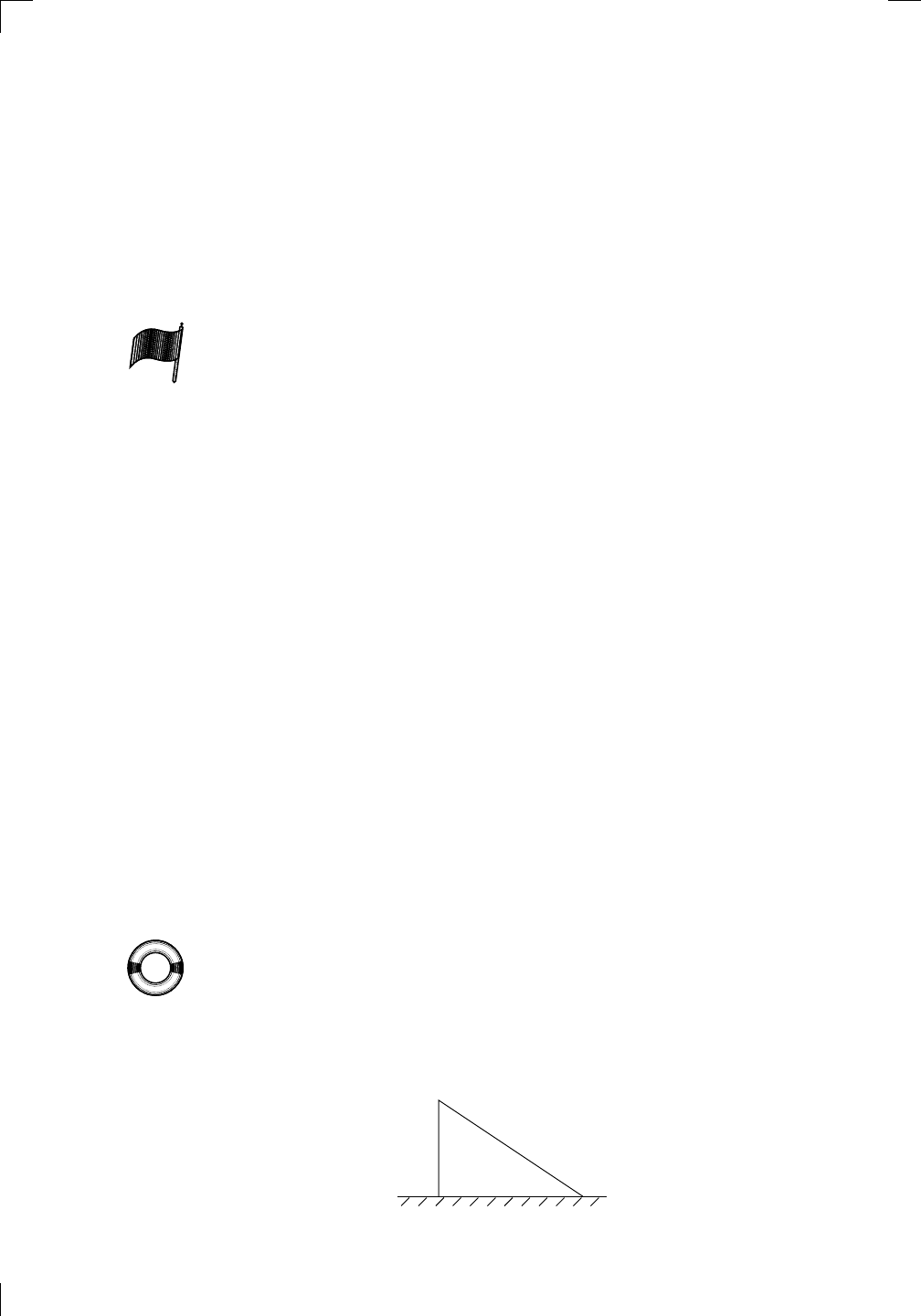
long, straight fence, and that the farmer wants to fence off a little enclosure
for some horses to graze in. The farmer is a little eccentric and would like to
make the enclosure in the shape of a right-angled triangle with the existing
fence as one of the sides which is not the hypotenuse, like this:
PSfrag
replacements
(
a, b)
[
a, b]
(
a, b]
[
a, b)
(
a, ∞)
[
a, ∞)
(
−∞, b)
(
−∞, b]
(
−∞, ∞)
{
x : a < x < b}
{
x : a ≤ x ≤ b}
{
x : a < x ≤ b}
{
x : a ≤ x < b}
{
x : x ≥ a}
{
x : x > a}
{
x : x ≤ b}
{
x : x < b}
R
a
b
shado
w
0
1
4
−
2
3
−
3
g(
x) = x
2
f(
x) = x
3
g(
x) = x
2
f(
x) = x
3
mirror
(y = x)
f
−
1
(x) =
3
√
x
y = h
(x)
y = h
−
1
(x)
y =
(x − 1)
2
−
1
x
Same
height
−
x
Same
length,
opp
osite signs
y = −
2x
−
2
1
y =
1
2
x − 1
2
−
1
y =
2
x
y =
10
x
y =
2
−x
y =
log
2
(x)
4
3
units
mirror
(x-axis)
y = |
x|
y = |
log
2
(x)|
θ radians
θ units
30
◦
=
π
6
45
◦
=
π
4
60
◦
=
π
3
120
◦
=
2
π
3
135
◦
=
3
π
4
150
◦
=
5
π
6
90
◦
=
π
2
180
◦
= π
210
◦
=
7
π
6
225
◦
=
5
π
4
240
◦
=
4
π
3
270
◦
=
3
π
2
300
◦
=
5
π
3
315
◦
=
7
π
4
330
◦
=
11
π
6
0
◦
=
0 radians
θ
hypotenuse
opp
osite
adjacen
t
0
(≡ 2π)
π
2
π
3
π
2
I
I
I
I
II
IV
θ
(
x, y)
x
y
r
7
π
6
reference
angle
reference
angle =
π
6
sin
+
sin −
cos
+
cos −
tan
+
tan −
A
S
T
C
7
π
4
9
π
13
5
π
6
(this
angle is
5π
6
clo
ckwise)
1
2
1
2
3
4
5
6
0
−
1
−
2
−
3
−
4
−
5
−
6
−
3π
−
5
π
2
−
2π
−
3
π
2
−
π
−
π
2
3
π
3
π
5
π
2
2
π
3
π
2
π
π
2
y =
sin(x)
1
0
−
1
−
3π
−
5
π
2
−
2π
−
3
π
2
−
π
−
π
2
3
π
5
π
2
2
π
2
π
3
π
2
π
π
2
y =
sin(x)
y =
cos(x)
−
π
2
π
2
y =
tan(x), −
π
2
<
x <
π
2
0
−
π
2
π
2
y =
tan(x)
−
2π
−
3π
−
5
π
2
−
3
π
2
−
π
−
π
2
π
2
3
π
3
π
5
π
2
2
π
3
π
2
π
y =
sec(x)
y =
csc(x)
y =
cot(x)
y = f(
x)
−
1
1
2
y = g(
x)
3
y = h
(x)
4
5
−
2
f(
x) =
1
x
g(
x) =
1
x
2
etc.
0
1
π
1
2
π
1
3
π
1
4
π
1
5
π
1
6
π
1
7
π
g(
x) = sin
1
x
1
0
−
1
L
10
100
200
y =
π
2
y = −
π
2
y =
tan
−1
(x)
π
2
π
y =
sin(
x)
x
,
x > 3
0
1
−
1
a
L
f(
x) = x sin (1/x)
(0 <
x < 0.3)
h
(x) = x
g(
x) = −x
a
L
lim
x
→a
+
f(x) = L
lim
x
→a
+
f(x) = ∞
lim
x
→a
+
f(x) = −∞
lim
x
→a
+
f(x) DNE
lim
x
→a
−
f(x) = L
lim
x
→a
−
f(x) = ∞
lim
x
→a
−
f(x) = −∞
lim
x
→a
−
f(x) DNE
M
}
lim
x
→a
−
f(x) = M
lim
x
→a
f(x) = L
lim
x
→a
f(x) DNE
lim
x
→∞
f(x) = L
lim
x
→∞
f(x) = ∞
lim
x
→∞
f(x) = −∞
lim
x
→∞
f(x) DNE
lim
x
→−∞
f(x) = L
lim
x
→−∞
f(x) = ∞
lim
x
→−∞
f(x) = −∞
lim
x
→−∞
f(x) DNE
lim
x →a
+
f(
x) = ∞
lim
x →a
+
f(
x) = −∞
lim
x →a
−
f(
x) = ∞
lim
x →a
−
f(
x) = −∞
lim
x →a
f(
x) = ∞
lim
x →a
f(
x) = −∞
lim
x →a
f(
x) DNE
y = f(
x)
a
y =
|
x|
x
1
−
1
y =
|
x + 2|
x +
2
1
−
1
−
2
1
2
3
4
a
a
b
y = x sin
1
x
y = x
y = −
x
a
b
c
d
C
a
b
c
d
−
1
0
1
2
3
time
y
t
u
(
t, f(t))
(
u, f(u))
time
y
t
u
y
x
(
x, f(x))
y = |
x|
(
z, f(z))
z
y = f(
x)
a
tangen
t at x = a
b
tangen
t at x = b
c
tangen
t at x = c
y = x
2
tangen
t
at x = −
1
u
v
uv
u +
∆u
v +
∆v
(
u + ∆u)(v + ∆v)
∆
u
∆
v
u
∆v
v∆
u
∆
u∆v
y = f(
x)
1
2
−
2
y = |
x
2
− 4|
y = x
2
− 4
y = −
2x + 5
y = g(
x)
1
2
3
4
5
6
7
8
9
0
−
1
−
2
−
3
−
4
−
5
−
6
y = f(
x)
3
−
3
3
−
3
0
−
1
2
easy
hard
flat
y = f
0
(
x)
3
−
3
0
−
1
2
1
−
1
y =
sin(x)
y = x
x
A
B
O
1
C
D
sin(
x)
tan(
x)
y =
sin
(x)
x
π
2
π
1
−
1
x =
0
a =
0
x
> 0
a
> 0
x
< 0
a
< 0
rest
position
+
−
y = x
2
sin
1
x
N
A
B
H
a
b
c
O
H
A
B
C
D
h
r
R
θ
1000
2000
α
β
p
h
y = g(
x) = log
b
(x)
y = f(
x) = b
x
y = e
x
5
10
1
2
3
4
0
−
1
−
2
−
3
−
4
y =
ln(x)
y =
cosh(x)
y =
sinh(x)
y =
tanh(x)
y =
sech(x)
y =
csch(x)
y =
coth(x)
1
−
1
y = f(
x)
original
function
in
verse function
slop
e = 0 at (x, y)
slop
e is infinite at (y, x)
−
108
2
5
1
2
1
2
3
4
5
6
0
−
1
−
2
−
3
−
4
−
5
−
6
−
3π
−
5
π
2
−
2π
−
3
π
2
−
π
−
π
2
3
π
3
π
5
π
2
2
π
3
π
2
π
π
2
y =
sin(x)
1
0
−
1
−
3π
−
5
π
2
−
2π
−
3
π
2
−
π
−
π
2
3
π
5
π
2
2
π
2
π
3
π
2
π
π
2
y =
sin(x)
y =
sin(x), −
π
2
≤ x ≤
π
2
−
2
−
1
0
2
π
2
−
π
2
y =
sin
−1
(x)
y =
cos(x)
π
π
2
y =
cos
−1
(x)
−
π
2
1
x
α
β
y =
tan(x)
y =
tan(x)
1
y =
tan
−1
(x)
y =
sec(x)
y =
sec
−1
(x)
y =
csc
−1
(x)
y =
cot
−1
(x)
1
y =
cosh
−1
(x)
y =
sinh
−1
(x)
y =
tanh
−1
(x)
y =
sech
−1
(x)
y =
csch
−1
(x)
y =
coth
−1
(x)
(0
, 3)
(2
, −1)
(5
, 2)
(7
, 0)
(
−1, 44)
(0
, 1)
(1
, −12)
(2
, 305)
y =
1
2
(2
, 3)
y = f(
x)
y = g(
x)
a
b
c
a
b
c
s
c
0
c
1
(
a, f(a))
(
b, f(b))
1
2
1
2
3
4
5
6
0
−
1
−
2
−
3
−
4
−
5
−
6
−
3π
−
5
π
2
−
2π
−
3
π
2
−
π
−
π
2
3
π
3
π
5
π
2
2
π
3
π
2
π
π
2
y = sin(x)
1
0
−1
−3π
−
5π
2
−2π
−
3π
2
−π
−
π
2
3π
5π
2
2π
2π
3π
2
π
π
2
c
OR
Local maximum
Local minimum
Horizontal point of inflection
1
e
y = f
0
(x)
y = f(x) = x ln(x)
−
1
e
?
y = f (x) = x
3
y = g(x) = x
4
x
f(x)
−3
−2
−1
0
1
2
1
2
3
4
+
−
?
1
5
6
3
f
0
(x)
2 −
1
2
√
6
2 +
1
2
√
6
f
00
(x)
7
8
g
00
(x)
f
00
(x)
0
y =
(x − 3)(x − 1)
2
x
3
(x + 2)
y = x ln(x)
1
e
−
1
e
5
−108
2
α
β
2 −
1
2
√
6
2 +
1
2
√
6
y = x
2
(x − 5)
3
−
e
−1/2
√
3
e
−1/2
√
3
−e
−3/2
e
−3/2
−
1
√
3
1
√
3
−1
1
y = xe
−3x
2
/2
y =
x
3
− 6x
2
+ 13x − 8
x
28
2
600
500
400
300
200
100
0
−100
−200
−300
−400
−500
−600
0
10
−10
5
−5
20
−20
15
−15
0
4
5
6
x
P
0
(x)
+
−
−
existing fence
new fence
enclosure
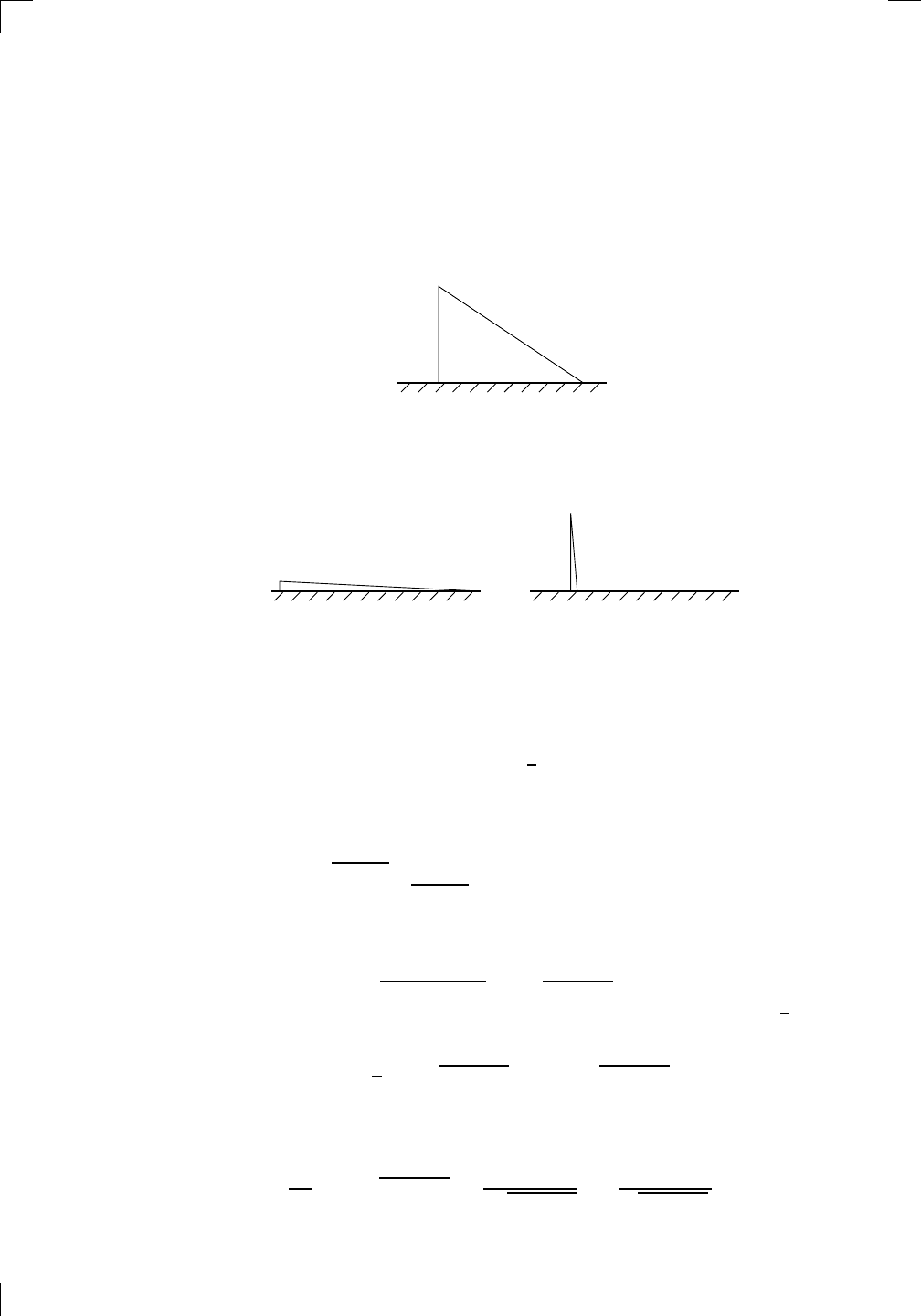
270 • Optimization and Linearization
Assuming that only 300 feet of fencing are available, and that the farmer wants
the enclosure to have the largest possible area, what are the dimensions and
area of the enclosure?
Let’s pick some variables. We’ll let the base of the triangle be b, the height
be h, the hypotenuse be H (all in feet), and the area be A (in square feet),
like this:
PSfrag
replacements
(
a, b)
[
a, b]
(
a, b]
[
a, b)
(
a, ∞)
[
a, ∞)
(
−∞, b)
(
−∞, b]
(
−∞, ∞)
{
x : a < x < b}
{
x : a ≤ x ≤ b}
{
x : a < x ≤ b}
{
x : a ≤ x < b}
{
x : x ≥ a}
{
x : x > a}
{
x : x ≤ b}
{
x : x < b}
R
a
b
shado
w
0
1
4
−
2
3
−
3
g(
x) = x
2
f(
x) = x
3
g(
x) = x
2
f(
x) = x
3
mirror
(y = x)
f
−
1
(x) =
3
√
x
y = h
(x)
y = h
−
1
(x)
y =
(x − 1)
2
−
1
x
Same
height
−
x
Same
length,
opp
osite signs
y = −
2x
−
2
1
y =
1
2
x − 1
2
−
1
y =
2
x
y =
10
x
y =
2
−x
y =
log
2
(x)
4
3
units
mirror
(x-axis)
y = |
x|
y = |
log
2
(x)|
θ radians
θ units
30
◦
=
π
6
45
◦
=
π
4
60
◦
=
π
3
120
◦
=
2
π
3
135
◦
=
3
π
4
150
◦
=
5
π
6
90
◦
=
π
2
180
◦
= π
210
◦
=
7
π
6
225
◦
=
5
π
4
240
◦
=
4
π
3
270
◦
=
3
π
2
300
◦
=
5
π
3
315
◦
=
7
π
4
330
◦
=
11
π
6
0
◦
=
0 radians
θ
hypotenuse
opp
osite
adjacen
t
0
(≡ 2π)
π
2
π
3
π
2
I
I
I
I
II
IV
θ
(
x, y)
x
y
r
7
π
6
reference
angle
reference
angle =
π
6
sin
+
sin −
cos
+
cos −
tan
+
tan −
A
S
T
C
7
π
4
9
π
13
5
π
6
(this
angle is
5π
6
clo
ckwise)
1
2
1
2
3
4
5
6
0
−
1
−
2
−
3
−
4
−
5
−
6
−
3π
−
5
π
2
−
2π
−
3
π
2
−
π
−
π
2
3
π
3
π
5
π
2
2
π
3
π
2
π
π
2
y =
sin(x)
1
0
−
1
−
3π
−
5
π
2
−
2π
−
3
π
2
−
π
−
π
2
3
π
5
π
2
2
π
2
π
3
π
2
π
π
2
y =
sin(x)
y =
cos(x)
−
π
2
π
2
y =
tan(x), −
π
2
<
x <
π
2
0
−
π
2
π
2
y =
tan(x)
−
2π
−
3π
−
5
π
2
−
3
π
2
−
π
−
π
2
π
2
3
π
3
π
5
π
2
2
π
3
π
2
π
y =
sec(x)
y =
csc(x)
y =
cot(x)
y = f(
x)
−
1
1
2
y = g(
x)
3
y = h
(x)
4
5
−
2
f(
x) =
1
x
g(
x) =
1
x
2
etc.
0
1
π
1
2
π
1
3
π
1
4
π
1
5
π
1
6
π
1
7
π
g(
x) = sin
1
x
1
0
−
1
L
10
100
200
y =
π
2
y = −
π
2
y =
tan
−1
(x)
π
2
π
y =
sin(
x)
x
,
x > 3
0
1
−
1
a
L
f(
x) = x sin (1/x)
(0 <
x < 0.3)
h
(x) = x
g(
x) = −x
a
L
lim
x
→a
+
f(x) = L
lim
x
→a
+
f(x) = ∞
lim
x
→a
+
f(x) = −∞
lim
x
→a
+
f(x) DNE
lim
x
→a
−
f(x) = L
lim
x
→a
−
f(x) = ∞
lim
x
→a
−
f(x) = −∞
lim
x
→a
−
f(x) DNE
M
}
lim
x
→a
−
f(x) = M
lim
x
→a
f(x) = L
lim
x
→a
f(x) DNE
lim
x
→∞
f(x) = L
lim
x
→∞
f(x) = ∞
lim
x
→∞
f(x) = −∞
lim
x
→∞
f(x) DNE
lim
x
→−∞
f(x) = L
lim
x
→−∞
f(x) = ∞
lim
x
→−∞
f(x) = −∞
lim
x
→−∞
f(x) DNE
lim
x →a
+
f(
x) = ∞
lim
x →a
+
f(
x) = −∞
lim
x →a
−
f(
x) = ∞
lim
x →a
−
f(
x) = −∞
lim
x →a
f(
x) = ∞
lim
x →a
f(
x) = −∞
lim
x →a
f(
x) DNE
y = f(
x)
a
y =
|
x|
x
1
−
1
y =
|
x + 2|
x +
2
1
−
1
−
2
1
2
3
4
a
a
b
y = x sin
1
x
y = x
y = −
x
a
b
c
d
C
a
b
c
d
−
1
0
1
2
3
time
y
t
u
(
t, f(t))
(
u, f(u))
time
y
t
u
y
x
(
x, f(x))
y = |
x|
(
z, f(z))
z
y = f(
x)
a
tangen
t at x = a
b
tangen
t at x = b
c
tangen
t at x = c
y = x
2
tangen
t
at x = −
1
u
v
uv
u +
∆u
v +
∆v
(
u + ∆u)(v + ∆v)
∆
u
∆
v
u
∆v
v∆
u
∆
u∆v
y = f(
x)
1
2
−
2
y = |
x
2
− 4|
y = x
2
− 4
y = −
2x + 5
y = g(
x)
1
2
3
4
5
6
7
8
9
0
−
1
−
2
−
3
−
4
−
5
−
6
y = f(
x)
3
−
3
3
−
3
0
−
1
2
easy
hard
flat
y = f
0
(
x)
3
−
3
0
−
1
2
1
−
1
y =
sin(x)
y = x
x
A
B
O
1
C
D
sin(
x)
tan(
x)
y =
sin
(x)
x
π
2
π
1
−
1
x =
0
a =
0
x
> 0
a
> 0
x
< 0
a
< 0
rest
position
+
−
y = x
2
sin
1
x
N
A
B
H
a
b
c
O
H
A
B
C
D
h
r
R
θ
1000
2000
α
β
p
h
y = g(
x) = log
b
(x)
y = f(
x) = b
x
y = e
x
5
10
1
2
3
4
0
−
1
−
2
−
3
−
4
y =
ln(x)
y =
cosh(x)
y =
sinh(x)
y =
tanh(x)
y =
sech(x)
y =
csch(x)
y =
coth(x)
1
−
1
y = f(
x)
original
function
in
verse function
slop
e = 0 at (x, y)
slop
e is infinite at (y, x)
−
108
2
5
1
2
1
2
3
4
5
6
0
−
1
−
2
−
3
−
4
−
5
−
6
−
3π
−
5
π
2
−
2π
−
3
π
2
−
π
−
π
2
3
π
3
π
5
π
2
2
π
3
π
2
π
π
2
y =
sin(x)
1
0
−
1
−
3π
−
5
π
2
−
2π
−
3
π
2
−
π
−
π
2
3
π
5
π
2
2
π
2
π
3
π
2
π
π
2
y =
sin(x)
y =
sin(x), −
π
2
≤ x ≤
π
2
−
2
−
1
0
2
π
2
−
π
2
y =
sin
−1
(x)
y =
cos(x)
π
π
2
y =
cos
−1
(x)
−
π
2
1
x
α
β
y =
tan(x)
y =
tan(x)
1
y =
tan
−1
(x)
y =
sec(x)
y =
sec
−1
(x)
y =
csc
−1
(x)
y =
cot
−1
(x)
1
y =
cosh
−1
(x)
y =
sinh
−1
(x)
y =
tanh
−1
(x)
y =
sech
−1
(x)
y =
csch
−1
(x)
y =
coth
−1
(x)
(0
, 3)
(2
, −1)
(5
, 2)
(7
, 0)
(
−1, 44)
(0
, 1)
(1
, −12)
(2
, 305)
y =
1
2
(2
, 3)
y = f(
x)
y = g(
x)
a
b
c
a
b
c
s
c
0
c
1
(
a, f(a))
(
b, f(b))
1
2
1
2
3
4
5
6
0
−
1
−
2
−
3
−
4
−
5
−
6
−
3π
−
5
π
2
−
2π
−
3
π
2
−
π
−
π
2
3
π
3
π
5
π
2
2
π
3
π
2
π
π
2
y =
sin(x)
1
0
−
1
−
3π
−
5
π
2
−
2π
−
3
π
2
−
π
−
π
2
3
π
5
π
2
2
π
2
π
3
π
2
π
π
2
c
OR
Lo
cal maximum
Lo
cal minimum
Horizon
tal point of inflection
1
e
y = f
0
(
x)
y = f(
x) = x ln(x)
−
1
e
?
y = f (
x) = x
3
y = g(
x) = x
4
x
f(
x)
−
3
−
2
−
1
0
1
2
1
2
3
4
+
−
?
1
5
6
3
f
0
(x)
2 −
1
2
√
6
2 +
1
2
√
6
f
00
(x)
7
8
g
00
(x)
f
00
(x)
0
y =
(x − 3)(x − 1)
2
x
3
(x + 2)
y = x ln(x)
1
e
−
1
e
5
−108
2
α
β
2 −
1
2
√
6
2 +
1
2
√
6
y = x
2
(x − 5)
3
−
e
−1/2
√
3
e
−1/2
√
3
−e
−3/2
e
−3/2
−
1
√
3
1
√
3
−1
1
y = xe
−3x
2
/2
y =
x
3
− 6x
2
+ 13x − 8
x
28
2
600
500
400
300
200
100
0
−100
−200
−300
−400
−500
−600
0
10
−10
5
−5
20
−20
15
−15
0
4
5
6
x
P
0
(x)
+
−
−
existing fence
new fence
enclosure
A
h
b
H
Note that the fence is of length h + H, and we want to maximize A. That
completes step 1. Moving on to the second step, consider some extreme shapes
that you can make out of 300 feet of fencing:
PSfrag
replacements
(
a, b)
[
a, b]
(
a, b]
[
a, b)
(
a, ∞)
[
a, ∞)
(
−∞, b)
(
−∞, b]
(
−∞, ∞)
{
x : a < x < b}
{
x : a ≤ x ≤ b}
{
x : a < x ≤ b}
{
x : a ≤ x < b}
{
x : x ≥ a}
{
x : x > a}
{
x : x ≤ b}
{
x : x < b}
R
a
b
shado
w
0
1
4
−
2
3
−
3
g(
x) = x
2
f(
x) = x
3
g(
x) = x
2
f(
x) = x
3
mirror
(y = x)
f
−
1
(x) =
3
√
x
y = h
(x)
y = h
−
1
(x)
y =
(x − 1)
2
−
1
x
Same
height
−
x
Same
length,
opp
osite signs
y = −
2x
−
2
1
y =
1
2
x − 1
2
−
1
y =
2
x
y =
10
x
y =
2
−x
y =
log
2
(x)
4
3
units
mirror
(x-axis)
y = |
x|
y = |
log
2
(x)|
θ radians
θ units
30
◦
=
π
6
45
◦
=
π
4
60
◦
=
π
3
120
◦
=
2
π
3
135
◦
=
3
π
4
150
◦
=
5
π
6
90
◦
=
π
2
180
◦
= π
210
◦
=
7
π
6
225
◦
=
5
π
4
240
◦
=
4
π
3
270
◦
=
3
π
2
300
◦
=
5
π
3
315
◦
=
7
π
4
330
◦
=
11
π
6
0
◦
=
0 radians
θ
hypotenuse
opp
osite
adjacen
t
0
(≡ 2π)
π
2
π
3
π
2
I
I
I
I
II
IV
θ
(
x, y)
x
y
r
7
π
6
reference
angle
reference
angle =
π
6
sin
+
sin −
cos
+
cos −
tan
+
tan −
A
S
T
C
7
π
4
9
π
13
5
π
6
(this
angle is
5π
6
clo
ckwise)
1
2
1
2
3
4
5
6
0
−
1
−
2
−
3
−
4
−
5
−
6
−
3π
−
5
π
2
−
2π
−
3
π
2
−
π
−
π
2
3
π
3
π
5
π
2
2
π
3
π
2
π
π
2
y =
sin(x)
1
0
−
1
−
3π
−
5
π
2
−
2π
−
3
π
2
−
π
−
π
2
3
π
5
π
2
2
π
2
π
3
π
2
π
π
2
y =
sin(x)
y =
cos(x)
−
π
2
π
2
y =
tan(x), −
π
2
<
x <
π
2
0
−
π
2
π
2
y =
tan(x)
−
2π
−
3π
−
5
π
2
−
3
π
2
−
π
−
π
2
π
2
3
π
3
π
5
π
2
2
π
3
π
2
π
y =
sec(x)
y =
csc(x)
y =
cot(x)
y = f(
x)
−
1
1
2
y = g(
x)
3
y = h
(x)
4
5
−
2
f(
x) =
1
x
g(
x) =
1
x
2
etc.
0
1
π
1
2
π
1
3
π
1
4
π
1
5
π
1
6
π
1
7
π
g(
x) = sin
1
x
1
0
−
1
L
10
100
200
y =
π
2
y = −
π
2
y =
tan
−1
(x)
π
2
π
y =
sin(
x)
x
,
x > 3
0
1
−
1
a
L
f(
x) = x sin (1/x)
(0 <
x < 0.3)
h
(x) = x
g(
x) = −x
a
L
lim
x
→a
+
f(x) = L
lim
x
→a
+
f(x) = ∞
lim
x
→a
+
f(x) = −∞
lim
x
→a
+
f(x) DNE
lim
x
→a
−
f(x) = L
lim
x
→a
−
f(x) = ∞
lim
x
→a
−
f(x) = −∞
lim
x
→a
−
f(x) DNE
M
}
lim
x
→a
−
f(x) = M
lim
x
→a
f(x) = L
lim
x
→a
f(x) DNE
lim
x
→∞
f(x) = L
lim
x
→∞
f(x) = ∞
lim
x
→∞
f(x) = −∞
lim
x
→∞
f(x) DNE
lim
x
→−∞
f(x) = L
lim
x
→−∞
f(x) = ∞
lim
x
→−∞
f(x) = −∞
lim
x
→−∞
f(x) DNE
lim
x →a
+
f(
x) = ∞
lim
x →a
+
f(
x) = −∞
lim
x →a
−
f(
x) = ∞
lim
x →a
−
f(
x) = −∞
lim
x →a
f(
x) = ∞
lim
x →a
f(
x) = −∞
lim
x →a
f(
x) DNE
y = f(
x)
a
y =
|
x|
x
1
−
1
y =
|
x + 2|
x +
2
1
−
1
−
2
1
2
3
4
a
a
b
y = x sin
1
x
y = x
y = −
x
a
b
c
d
C
a
b
c
d
−
1
0
1
2
3
time
y
t
u
(
t, f(t))
(
u, f(u))
time
y
t
u
y
x
(
x, f(x))
y = |
x|
(
z, f(z))
z
y = f(
x)
a
tangen
t at x = a
b
tangen
t at x = b
c
tangen
t at x = c
y = x
2
tangen
t
at x = −
1
u
v
uv
u +
∆u
v +
∆v
(
u + ∆u)(v + ∆v)
∆
u
∆
v
u
∆v
v∆
u
∆
u∆v
y = f(
x)
1
2
−
2
y = |
x
2
− 4|
y = x
2
− 4
y = −
2x + 5
y = g(
x)
1
2
3
4
5
6
7
8
9
0
−
1
−
2
−
3
−
4
−
5
−
6
y = f(
x)
3
−
3
3
−
3
0
−
1
2
easy
hard
flat
y = f
0
(
x)
3
−
3
0
−
1
2
1
−
1
y =
sin(x)
y = x
x
A
B
O
1
C
D
sin(
x)
tan(
x)
y =
sin
(x)
x
π
2
π
1
−
1
x =
0
a =
0
x
> 0
a
> 0
x
< 0
a
< 0
rest
position
+
−
y = x
2
sin
1
x
N
A
B
H
a
b
c
O
H
A
B
C
D
h
r
R
θ
1000
2000
α
β
p
h
y = g(
x) = log
b
(x)
y = f(
x) = b
x
y = e
x
5
10
1
2
3
4
0
−
1
−
2
−
3
−
4
y =
ln(x)
y =
cosh(x)
y =
sinh(x)
y =
tanh(x)
y =
sech(x)
y =
csch(x)
y =
coth(x)
1
−
1
y = f(
x)
original
function
in
verse function
slop
e = 0 at (x, y)
slop
e is infinite at (y, x)
−
108
2
5
1
2
1
2
3
4
5
6
0
−
1
−
2
−
3
−
4
−
5
−
6
−
3π
−
5
π
2
−
2π
−
3
π
2
−
π
−
π
2
3
π
3
π
5
π
2
2
π
3
π
2
π
π
2
y =
sin(x)
1
0
−
1
−
3π
−
5
π
2
−
2π
−
3
π
2
−
π
−
π
2
3
π
5
π
2
2
π
2
π
3
π
2
π
π
2
y =
sin(x)
y =
sin(x), −
π
2
≤ x ≤
π
2
−
2
−
1
0
2
π
2
−
π
2
y =
sin
−1
(x)
y =
cos(x)
π
π
2
y =
cos
−1
(x)
−
π
2
1
x
α
β
y =
tan(x)
y =
tan(x)
1
y =
tan
−1
(x)
y =
sec(x)
y =
sec
−1
(x)
y =
csc
−1
(x)
y =
cot
−1
(x)
1
y =
cosh
−1
(x)
y =
sinh
−1
(x)
y =
tanh
−1
(x)
y =
sech
−1
(x)
y =
csch
−1
(x)
y =
coth
−1
(x)
(0
, 3)
(2
, −1)
(5
, 2)
(7
, 0)
(
−1, 44)
(0
, 1)
(1
, −12)
(2
, 305)
y =
1
2
(2
, 3)
y = f(
x)
y = g(
x)
a
b
c
a
b
c
s
c
0
c
1
(
a, f(a))
(
b, f(b))
1
2
1
2
3
4
5
6
0
−
1
−
2
−
3
−
4
−
5
−
6
−
3π
−
5
π
2
−
2π
−
3
π
2
−
π
−
π
2
3
π
3
π
5
π
2
2
π
3
π
2
π
π
2
y =
sin(x)
1
0
−
1
−
3π
−
5
π
2
−
2π
−
3
π
2
−
π
−
π
2
3
π
5
π
2
2
π
2
π
3
π
2
π
π
2
c
OR
Lo
cal maximum
Lo
cal minimum
Horizon
tal point of inflection
1
e
y = f
0
(
x)
y = f(
x) = x ln(x)
−
1
e
?
y = f (
x) = x
3
y = g(
x) = x
4
x
f(
x)
−3
−2
−1
0
1
2
1
2
3
4
+
−
?
1
5
6
3
f
0
(x)
2 −
1
2
√
6
2 +
1
2
√
6
f
00
(x)
7
8
g
00
(x)
f
00
(x)
0
y =
(x − 3)(x − 1)
2
x
3
(x + 2)
y = x ln(x)
1
e
−
1
e
5
−108
2
α
β
2 −
1
2
√
6
2 +
1
2
√
6
y = x
2
(x − 5)
3
−
e
−1/2
√
3
e
−1/2
√
3
−e
−3/2
e
−3/2
−
1
√
3
1
√
3
−1
1
y = xe
−3x
2
/2
y =
x
3
− 6x
2
+ 13x − 8
x
28
2
600
500
400
300
200
100
0
−100
−200
−300
−400
−500
−600
0
10
−10
5
−5
20
−20
15
−15
0
4
5
6
x
P
0
(x)
+
−
−
existing fence
new fence
enclosure
A
h
h
b
b
H
H
In the first case, h is nearly 0, while b and H are both almost 300, but the area
is tiny! In the second case, b is nearly 0, while h and H are both almost 150.
The area is still very small. So we can do better by some middle-of-the-road
solution. We have at least determined that b and H are between 0 and 300,
and that h is between 0 and 150.
Moving on to step 3, we see that A =
1
2
bh and also that h + H = 300. We
still need one more equation, since we have to condense the three variables b,
h, and H down to one. In fact, we can use Pythagoras’ Theorem to say that
b
2
+ h
2
= H
2
.
Now we should try to eliminate some variables. We can take square roots
and write H =
√
b
2
+ h
2
, since we know H > 0; substituting into h+H = 300,
we get the equation h +
√
b
2
+ h
2
= 300. Let’s try to eliminate b from this.
Subtract h from both sides and square to get
b
2
+ h
2
= (300 − h)
2
= 90000 − 600h + h
2
.
This means that b =
√
90000 − 600h = 10
√
900 − 6h, again since b is positive
(that is, it can’t be the negative square root!). Finally, the equation A =
1
2
bh
can be rewritten as
A =
1
2
× 10
√
900 − 6h × h = 5h
√
900 − 6h,
where h lies in the interval [0, 150]. That’s step 4. As for step 5, you can use
the product rule and the chain rule to see that
dA
dh
= 5
√
900 − 6h + h
−6
2
√
900 − 6h
=
45(100 − h)
√
900 − 6h
.
Section 13.1.4: Another optimization example • 271
This equals 0 when 100 −h = 0, that is, when h = 100. Moving on to step 6,
we substitute h = 100 into the equation for A above, and we get
A = 5(100)
p
900 − 6(100) = 500
√
300 = 5000
√
3.
On the other hand, at the endpoint h = 0, we see that A = 0; similarly, when
h = 150, the quantity 900 −6h vanishes, so A = 0 once again. The conclusion
is that A is maximized when h = 100. We can check this with a table of signs.
This isn’t so bad, since the numerator of dA/dh is just 45(100 −h), while the
denominator is always positive. The table of signs for dA/dh looks like this:
PSfrag
replacements
(
a, b)
[
a, b]
(
a, b]
[
a, b)
(
a, ∞)
[
a, ∞)
(
−∞, b)
(
−∞, b]
(
−∞, ∞)
{
x : a < x < b}
{
x : a ≤ x ≤ b}
{
x : a < x ≤ b}
{
x : a ≤ x < b}
{
x : x ≥ a}
{
x : x > a}
{
x : x ≤ b}
{
x : x < b}
R
a
b
shado
w
0
1
4
−
2
3
−
3
g(
x) = x
2
f(
x) = x
3
g(
x) = x
2
f(
x) = x
3
mirror
(y = x)
f
−
1
(x) =
3
√
x
y = h
(x)
y = h
−
1
(x)
y =
(x − 1)
2
−
1
x
Same
height
−
x
Same
length,
opp
osite signs
y = −
2x
−
2
1
y =
1
2
x − 1
2
−
1
y =
2
x
y =
10
x
y =
2
−x
y =
log
2
(x)
4
3
units
mirror
(x-axis)
y = |
x|
y = |
log
2
(x)|
θ radians
θ units
30
◦
=
π
6
45
◦
=
π
4
60
◦
=
π
3
120
◦
=
2
π
3
135
◦
=
3
π
4
150
◦
=
5
π
6
90
◦
=
π
2
180
◦
= π
210
◦
=
7
π
6
225
◦
=
5
π
4
240
◦
=
4
π
3
270
◦
=
3
π
2
300
◦
=
5
π
3
315
◦
=
7
π
4
330
◦
=
11
π
6
0
◦
=
0 radians
θ
hypotenuse
opp
osite
adjacen
t
0
(≡ 2π)
π
2
π
3
π
2
I
I
I
I
II
IV
θ
(
x, y)
x
y
r
7
π
6
reference
angle
reference
angle =
π
6
sin
+
sin −
cos
+
cos −
tan
+
tan −
A
S
T
C
7
π
4
9
π
13
5
π
6
(this
angle is
5π
6
clo
ckwise)
1
2
1
2
3
4
5
6
0
−
1
−
2
−
3
−
4
−
5
−
6
−
3π
−
5
π
2
−
2π
−
3
π
2
−
π
−
π
2
3
π
3
π
5
π
2
2
π
3
π
2
π
π
2
y =
sin(x)
1
0
−
1
−
3π
−
5
π
2
−
2π
−
3
π
2
−
π
−
π
2
3
π
5
π
2
2
π
2
π
3
π
2
π
π
2
y =
sin(x)
y =
cos(x)
−
π
2
π
2
y =
tan(x), −
π
2
<
x <
π
2
0
−
π
2
π
2
y =
tan(x)
−
2π
−
3π
−
5
π
2
−
3
π
2
−
π
−
π
2
π
2
3
π
3
π
5
π
2
2
π
3
π
2
π
y =
sec(x)
y =
csc(x)
y =
cot(x)
y = f (
x)
−
1
1
2
y = g(
x)
3
y = h
(x)
4
5
−
2
f(
x) =
1
x
g(
x) =
1
x
2
etc.
0
1
π
1
2
π
1
3
π
1
4
π
1
5
π
1
6
π
1
7
π
g(
x) = sin
1
x
1
0
−
1
L
10
100
200
y =
π
2
y = −
π
2
y =
tan
−1
(x)
π
2
π
y =
sin
(x)
x
,
x > 3
0
1
−
1
a
L
f(
x) = x sin (1/x)
(0 <
x < 0.3)
h
(x) = x
g(
x) = −x
a
L
lim
x
→a
+
f(x) = L
lim
x
→a
+
f(x) = ∞
lim
x
→a
+
f(x) = −∞
lim
x
→a
+
f(x) DNE
lim
x
→a
−
f(x) = L
lim
x
→a
−
f(x) = ∞
lim
x
→a
−
f(x) = −∞
lim
x
→a
−
f(x) DNE
M
}
lim
x
→a
−
f(x) = M
lim
x
→a
f(x) = L
lim
x
→a
f(x) DNE
lim
x
→∞
f(x) = L
lim
x
→∞
f(x) = ∞
lim
x
→∞
f(x) = −∞
lim
x
→∞
f(x) DNE
lim
x
→−∞
f(x) = L
lim
x
→−∞
f(x) = ∞
lim
x
→−∞
f(x) = −∞
lim
x
→−∞
f(x) DNE
lim
x →a
+
f(
x) = ∞
lim
x →a
+
f(
x) = −∞
lim
x →a
−
f(
x) = ∞
lim
x →a
−
f(
x) = −∞
lim
x →a
f(
x) = ∞
lim
x →a
f(
x) = −∞
lim
x →a
f(
x) DNE
y = f (
x)
a
y =
|
x|
x
1
−
1
y =
|
x + 2|
x +
2
1
−
1
−
2
1
2
3
4
a
a
b
y = x sin
1
x
y = x
y = −
x
a
b
c
d
C
a
b
c
d
−
1
0
1
2
3
time
y
t
u
(
t, f(t))
(
u, f(u))
time
y
t
u
y
x
(
x, f(x))
y = |
x|
(
z, f(z))
z
y = f (
x)
a
tangen
t at x = a
b
tangen
t at x = b
c
tangen
t at x = c
y = x
2
tangen
t
at x = −
1
u
v
uv
u +
∆u
v +
∆v
(
u + ∆u)(v + ∆v)
∆
u
∆
v
u
∆v
v∆
u
∆
u∆v
y = f (
x)
1
2
−
2
y = |
x
2
− 4|
y = x
2
− 4
y = −
2x + 5
y = g(
x)
1
2
3
4
5
6
7
8
9
0
−
1
−
2
−
3
−
4
−
5
−
6
y = f(
x)
3
−
3
3
−
3
0
−
1
2
easy
hard
flat
y = f
0
(
x)
3
−
3
0
−
1
2
1
−
1
y =
sin(x)
y = x
x
A
B
O
1
C
D
sin(
x)
tan(
x)
y =
sin
(x)
x
π
2
π
1
−
1
x =
0
a =
0
x
> 0
a
> 0
x
< 0
a
< 0
rest
position
+
−
y = x
2
sin
1
x
N
A
B
H
a
b
c
O
H
A
B
C
D
h
r
R
θ
1000
2000
α
β
p
h
y = g(
x) = log
b
(x)
y = f (
x) = b
x
y = e
x
5
10
1
2
3
4
0
−
1
−
2
−
3
−
4
y =
ln(x)
y =
cosh(x)
y =
sinh(x)
y =
tanh(x)
y =
sech(x)
y =
csch(x)
y =
coth(x)
1
−
1
y = f (
x)
original
function
in
verse function
slop
e = 0 at (x, y)
slop
e is infinite at (y, x)
−
108
2
5
1
2
1
2
3
4
5
6
0
−
1
−
2
−
3
−
4
−
5
−
6
−
3π
−
5
π
2
−
2π
−
3
π
2
−
π
−
π
2
3
π
3
π
5
π
2
2
π
3
π
2
π
π
2
y =
sin(x)
1
0
−
1
−
3π
−
5
π
2
−
2π
−
3
π
2
−
π
−
π
2
3
π
5
π
2
2
π
2
π
3
π
2
π
π
2
y =
sin(x)
y =
sin(x), −
π
2
≤ x ≤
π
2
−
2
−
1
0
2
π
2
−
π
2
y =
sin
−1
(x)
y =
cos(x)
π
π
2
y =
cos
−1
(x)
−
π
2
1
x
α
β
y =
tan(x)
y =
tan(x)
1
y =
tan
−1
(x)
y =
sec(x)
y =
sec
−1
(x)
y =
csc
−1
(x)
y =
cot
−1
(x)
1
y =
cosh
−1
(x)
y =
sinh
−1
(x)
y =
tanh
−1
(x)
y =
sech
−1
(x)
y =
csch
−1
(x)
y =
coth
−1
(x)
(0
, 3)
(2
, −1)
(5
, 2)
(7
, 0)
(
−1, 44)
(0
, 1)
(1
, −12)
(2
, 305)
y =
1
2
(2
, 3)
y = f (
x)
y = g(
x)
a
b
c
a
b
c
s
c
0
c
1
(
a, f(a))
(
b, f(b))
1
2
1
2
3
4
5
6
0
−
1
−
2
−
3
−
4
−
5
−
6
−
3π
−
5
π
2
−
2π
−
3
π
2
−
π
−
π
2
3
π
3
π
5
π
2
2
π
3
π
2
π
π
2
y =
sin(x)
1
0
−
1
−
3π
−
5
π
2
−
2π
−
3
π
2
−
π
−
π
2
3
π
5
π
2
2
π
2
π
3
π
2
π
π
2
c
OR
Lo
cal maximum
Lo
cal minimum
Horizon
tal point of inflection
1
e
y = f
0
(
x)
y = f(
x) = x ln(x)
−
1
e
?
y = f(
x) = x
3
y = g(
x) = x
4
x
f(
x)
−
3
−
2
−
1
0
1
2
1
2
3
4
+
−
?
1
5
6
3
f
0
(x)
2 −
1
2
√
6
2 +
1
2
√
6
f
00
(x)
7
8
g
00
(x)
f
00
(x)
0
y =
(x − 3)(x − 1)
2
x
3
(x + 2)
y = x ln(x)
1
e
−
1
e
5
−108
2
α
β
2 −
1
2
√
6
2 +
1
2
√
6
y = x
2
(x − 5)
3
−
e
−1/2
√
3
e
−1/2
√
3
−e
−3/2
e
−3/2
−
1
√
3
1
√
3
−1
1
y = xe
−3x
2
/2
y =
x
3
− 6x
2
+ 13x − 8
x
28
2
600
500
400
300
200
100
0
−100
−200
−300
−400
−500
−600
0
10
−10
5
−5
20
−20
15
−15
0
4
5
6
x
P
0
(x)
+
−
−
existing fence
new fence
enclosure
A
h
b
H
99 100 101h
dA/dh
So h = 100 is indeed a local maximum, as we suspected.
Now we just have to finish it off. The question asks for the dimensions,
and we only have one: h = 100. We’d better find b and H. Just look back at
the equations: we know that h + H = 300, so we immediately get H = 200.
Also, we know that b
2
+ h
2
= H
2
; plugging in h = 100 and H = 200,
we can see that b = 100
√
3. Finally, we already found that the maximum
value of A is 5000
√
3. So our concluding sentence could go something like
this: the enclosure of maximal area has base 100
√
3 feet, height 100 feet, and
hypotenuse 200 feet, and the area is then 5000
√
3 square feet.
13.1.4 Another optimization example
Here’s a nice problem. Suppose that you are manufacturing closed, hollow
PSfrag
replacements
(
a, b)
[
a, b]
(
a, b]
[
a, b)
(
a, ∞)
[
a, ∞)
(
−∞, b)
(
−∞, b]
(
−∞, ∞)
{
x : a < x < b}
{
x : a ≤ x ≤ b}
{
x : a < x ≤ b}
{
x : a ≤ x < b}
{
x : x ≥ a}
{
x : x > a}
{
x : x ≤ b}
{
x : x < b}
R
a
b
shado
w
0
1
4
−
2
3
−
3
g(
x) = x
2
f(
x) = x
3
g(
x) = x
2
f(
x) = x
3
mirror
(y = x)
f
−
1
(x) =
3
√
x
y = h
(x)
y = h
−
1
(x)
y =
(x − 1)
2
−
1
x
Same
height
−
x
Same
length,
opp
osite signs
y = −
2x
−
2
1
y =
1
2
x − 1
2
−
1
y =
2
x
y =
10
x
y =
2
−x
y =
log
2
(x)
4
3
units
mirror
(x-axis)
y = |
x|
y = |
log
2
(x)|
θ radians
θ units
30
◦
=
π
6
45
◦
=
π
4
60
◦
=
π
3
120
◦
=
2
π
3
135
◦
=
3
π
4
150
◦
=
5
π
6
90
◦
=
π
2
180
◦
= π
210
◦
=
7
π
6
225
◦
=
5
π
4
240
◦
=
4
π
3
270
◦
=
3
π
2
300
◦
=
5
π
3
315
◦
=
7
π
4
330
◦
=
11
π
6
0
◦
=
0 radians
θ
hypotenuse
opp
osite
adjacen
t
0
(≡ 2π)
π
2
π
3
π
2
I
I
I
I
II
IV
θ
(
x, y)
x
y
r
7
π
6
reference
angle
reference
angle =
π
6
sin
+
sin −
cos
+
cos −
tan
+
tan −
A
S
T
C
7
π
4
9
π
13
5
π
6
(this
angle is
5π
6
clo
ckwise)
1
2
1
2
3
4
5
6
0
−
1
−
2
−
3
−
4
−
5
−
6
−
3π
−
5
π
2
−
2π
−
3
π
2
−
π
−
π
2
3
π
3
π
5
π
2
2
π
3
π
2
π
π
2
y =
sin(x)
1
0
−
1
−
3π
−
5
π
2
−
2π
−
3
π
2
−
π
−
π
2
3
π
5
π
2
2
π
2
π
3
π
2
π
π
2
y =
sin(x)
y =
cos(x)
−
π
2
π
2
y =
tan(x), −
π
2
<
x <
π
2
0
−
π
2
π
2
y =
tan(x)
−
2π
−
3π
−
5
π
2
−
3
π
2
−
π
−
π
2
π
2
3
π
3
π
5
π
2
2
π
3
π
2
π
y =
sec(x)
y =
csc(x)
y =
cot(x)
y = f(
x)
−
1
1
2
y = g(
x)
3
y = h
(x)
4
5
−
2
f(
x) =
1
x
g(
x) =
1
x
2
etc.
0
1
π
1
2
π
1
3
π
1
4
π
1
5
π
1
6
π
1
7
π
g(
x) = sin
1
x
1
0
−
1
L
10
100
200
y =
π
2
y = −
π
2
y =
tan
−1
(x)
π
2
π
y =
sin(
x)
x
,
x > 3
0
1
−
1
a
L
f(
x) = x sin (1/x)
(0 <
x < 0.3)
h
(x) = x
g(
x) = −x
a
L
lim
x
→a
+
f(x) = L
lim
x
→a
+
f(x) = ∞
lim
x
→a
+
f(x) = −∞
lim
x
→a
+
f(x) DNE
lim
x
→a
−
f(x) = L
lim
x
→a
−
f(x) = ∞
lim
x
→a
−
f(x) = −∞
lim
x
→a
−
f(x) DNE
M
}
lim
x
→a
−
f(x) = M
lim
x
→a
f(x) = L
lim
x
→a
f(x) DNE
lim
x
→∞
f(x) = L
lim
x
→∞
f(x) = ∞
lim
x
→∞
f(x) = −∞
lim
x
→∞
f(x) DNE
lim
x
→−∞
f(x) = L
lim
x
→−∞
f(x) = ∞
lim
x
→−∞
f(x) = −∞
lim
x
→−∞
f(x) DNE
lim
x →a
+
f(
x) = ∞
lim
x →a
+
f(
x) = −∞
lim
x →a
−
f(
x) = ∞
lim
x →a
−
f(
x) = −∞
lim
x →a
f(
x) = ∞
lim
x →a
f(
x) = −∞
lim
x →a
f(
x) DNE
y = f (
x)
a
y =
|
x|
x
1
−
1
y =
|
x + 2|
x +
2
1
−
1
−
2
1
2
3
4
a
a
b
y = x sin
1
x
y = x
y = −
x
a
b
c
d
C
a
b
c
d
−
1
0
1
2
3
time
y
t
u
(
t, f(t))
(
u, f(u))
time
y
t
u
y
x
(
x, f(x))
y = |
x|
(
z, f(z))
z
y = f(
x)
a
tangen
t at x = a
b
tangen
t at x = b
c
tangen
t at x = c
y = x
2
tangen
t
at x = −
1
u
v
uv
u +
∆u
v +
∆v
(
u + ∆u)(v + ∆v)
∆
u
∆
v
u
∆v
v∆
u
∆
u∆v
y = f(
x)
1
2
−
2
y = |
x
2
− 4|
y = x
2
− 4
y = −
2x + 5
y = g(
x)
1
2
3
4
5
6
7
8
9
0
−
1
−
2
−
3
−
4
−
5
−
6
y = f (
x)
3
−
3
3
−
3
0
−
1
2
easy
hard
flat
y = f
0
(
x)
3
−
3
0
−
1
2
1
−
1
y =
sin(x)
y = x
x
A
B
O
1
C
D
sin(
x)
tan(
x)
y =
sin(
x)
x
π
2
π
1
−
1
x =
0
a =
0
x
> 0
a
> 0
x
< 0
a
< 0
rest
position
+
−
y = x
2
sin
1
x
N
A
B
H
a
b
c
O
H
A
B
C
D
h
r
R
θ
1000
2000
α
β
p
h
y = g(
x) = log
b
(x)
y = f(
x) = b
x
y = e
x
5
10
1
2
3
4
0
−
1
−
2
−
3
−
4
y =
ln(x)
y =
cosh(x)
y =
sinh(x)
y =
tanh(x)
y =
sech(x)
y =
csch(x)
y =
coth(x)
1
−
1
y = f(
x)
original
function
in
verse function
slop
e = 0 at (x, y)
slop
e is infinite at (y, x)
−
108
2
5
1
2
1
2
3
4
5
6
0
−
1
−
2
−
3
−
4
−
5
−
6
−
3π
−
5
π
2
−
2π
−
3
π
2
−
π
−
π
2
3
π
3
π
5
π
2
2
π
3
π
2
π
π
2
y =
sin(x)
1
0
−
1
−
3π
−
5
π
2
−
2π
−
3
π
2
−
π
−
π
2
3
π
5
π
2
2
π
2
π
3
π
2
π
π
2
y =
sin(x)
y =
sin(x), −
π
2
≤ x ≤
π
2
−
2
−
1
0
2
π
2
−
π
2
y =
sin
−1
(x)
y =
cos(x)
π
π
2
y =
cos
−1
(x)
−
π
2
1
x
α
β
y =
tan(x)
y =
tan(x)
1
y =
tan
−1
(x)
y =
sec(x)
y =
sec
−1
(x)
y =
csc
−1
(x)
y =
cot
−1
(x)
1
y =
cosh
−1
(x)
y =
sinh
−1
(x)
y =
tanh
−1
(x)
y =
sech
−1
(x)
y =
csch
−1
(x)
y =
coth
−1
(x)
(0
, 3)
(2
, −1)
(5
, 2)
(7
, 0)
(
−1, 44)
(0
, 1)
(1
, −12)
(2
, 305)
y =
1
2
(2
, 3)
y = f(
x)
y = g(
x)
a
b
c
a
b
c
s
c
0
c
1
(
a, f(a))
(
b, f(b))
1
2
1
2
3
4
5
6
0
−
1
−
2
−
3
−
4
−
5
−
6
−
3π
−
5
π
2
−
2π
−
3
π
2
−
π
−
π
2
3
π
3
π
5
π
2
2
π
3
π
2
π
π
2
y =
sin(x)
1
0
−
1
−
3π
−
5
π
2
−
2π
−
3
π
2
−
π
−
π
2
3
π
5
π
2
2
π
2
π
3
π
2
π
π
2
c
OR
Lo
cal maximum
Lo
cal minimum
Horizon
tal point of inflection
1
e
y = f
0
(
x)
y = f (
x) = x ln(x)
−
1
e
?
y = f(
x) = x
3
y = g(x) = x
4
x
f(x)
−3
−2
−1
0
1
2
1
2
3
4
+
−
?
1
5
6
3
f
0
(x)
2 −
1
2
√
6
2 +
1
2
√
6
f
00
(x)
7
8
g
00
(x)
f
00
(x)
0
y =
(x − 3)(x − 1)
2
x
3
(x + 2)
y = x ln(x)
1
e
−
1
e
5
−108
2
α
β
2 −
1
2
√
6
2 +
1
2
√
6
y = x
2
(x − 5)
3
−
e
−1/2
√
3
e
−1/2
√
3
−e
−3/2
e
−3/2
−
1
√
3
1
√
3
−1
1
y = xe
−3x
2
/2
y =
x
3
− 6x
2
+ 13x − 8
x
28
2
600
500
400
300
200
100
0
−100
−200
−300
−400
−500
−600
0
10
−10
5
−5
20
−20
15
−15
0
4
5
6
x
P
0
(x)
+
−
−
existing fence
new fence
enclosure
A
h
b
H
99
100
101
h
dA/dh
cylindrical metal cans. You can choose their dimensions, but the volume of
a can must be 16π cubic inches. You’d like to use as little metal as possible,
since the metal costs 2 cents per square inch. What dimensions should the
cans be to make your costs as low as possible, and how much does each can
cost in that case?
As a follow-up problem, how does the situation change if we now take
into account that the top and bottom of each can have to be welded onto the
curved bit, and it costs 14 cents an inch to weld?
Let’s start with the first part. Here’s a diagram of the situation:
PSfrag
replacements
(
a, b)
[
a, b]
(
a, b]
[
a, b)
(
a, ∞)
[
a, ∞)
(
−∞, b)
(
−∞, b]
(
−∞, ∞)
{
x : a < x < b}
{
x : a ≤ x ≤ b}
{
x : a < x ≤ b}
{
x : a ≤ x < b}
{
x : x ≥ a}
{
x : x > a}
{
x : x ≤ b}
{
x : x < b}
R
a
b
shado
w
0
1
4
−
2
3
−
3
g(
x) = x
2
f(
x) = x
3
g(
x) = x
2
f(
x) = x
3
mirror
(y = x)
f
−
1
(x) =
3
√
x
y = h
(x)
y = h
−
1
(x)
y =
(x − 1)
2
−
1
x
Same
height
−
x
Same
length,
opp
osite signs
y = −
2x
−
2
1
y =
1
2
x − 1
2
−
1
y =
2
x
y =
10
x
y =
2
−x
y =
log
2
(x)
4
3
units
mirror
(x-axis)
y = |
x|
y = |
log
2
(x)|
θ radians
θ units
30
◦
=
π
6
45
◦
=
π
4
60
◦
=
π
3
120
◦
=
2
π
3
135
◦
=
3
π
4
150
◦
=
5
π
6
90
◦
=
π
2
180
◦
= π
210
◦
=
7
π
6
225
◦
=
5
π
4
240
◦
=
4
π
3
270
◦
=
3
π
2
300
◦
=
5
π
3
315
◦
=
7
π
4
330
◦
=
11
π
6
0
◦
=
0 radians
θ
hypotenuse
opp
osite
adjacen
t
0
(≡ 2π)
π
2
π
3
π
2
I
I
I
I
II
IV
θ
(
x, y)
x
y
r
7
π
6
reference
angle
reference
angle =
π
6
sin
+
sin −
cos
+
cos −
tan
+
tan −
A
S
T
C
7
π
4
9
π
13
5
π
6
(this
angle is
5π
6
clo
ckwise)
1
2
1
2
3
4
5
6
0
−
1
−
2
−
3
−
4
−
5
−
6
−
3π
−
5
π
2
−
2π
−
3
π
2
−
π
−
π
2
3
π
3
π
5
π
2
2
π
3
π
2
π
π
2
y =
sin(x)
1
0
−
1
−
3π
−
5
π
2
−
2π
−
3
π
2
−
π
−
π
2
3
π
5
π
2
2
π
2
π
3
π
2
π
π
2
y =
sin(x)
y =
cos(x)
−
π
2
π
2
y =
tan(x), −
π
2
<
x <
π
2
0
−
π
2
π
2
y =
tan(x)
−
2π
−
3π
−
5
π
2
−
3
π
2
−
π
−
π
2
π
2
3
π
3
π
5
π
2
2
π
3
π
2
π
y =
sec(x)
y =
csc(x)
y =
cot(x)
y = f(
x)
−
1
1
2
y = g(
x)
3
y = h
(x)
4
5
−
2
f(
x) =
1
x
g(
x) =
1
x
2
etc.
0
1
π
1
2
π
1
3
π
1
4
π
1
5
π
1
6
π
1
7
π
g(
x) = sin
1
x
1
0
−
1
L
10
100
200
y =
π
2
y = −
π
2
y =
tan
−1
(x)
π
2
π
y =
sin(
x)
x
,
x > 3
0
1
−
1
a
L
f(
x) = x sin (1/x)
(0 <
x < 0.3)
h
(x) = x
g(
x) = −x
a
L
lim
x
→a
+
f(x) = L
lim
x
→a
+
f(x) = ∞
lim
x
→a
+
f(x) = −∞
lim
x
→a
+
f(x) DNE
lim
x
→a
−
f(x) = L
lim
x
→a
−
f(x) = ∞
lim
x
→a
−
f(x) = −∞
lim
x
→a
−
f(x) DNE
M
}
lim
x
→a
−
f(x) = M
lim
x
→a
f(x) = L
lim
x
→a
f(x) DNE
lim
x
→∞
f(x) = L
lim
x
→∞
f(x) = ∞
lim
x
→∞
f(x) = −∞
lim
x
→∞
f(x) DNE
lim
x
→−∞
f(x) = L
lim
x
→−∞
f(x) = ∞
lim
x
→−∞
f(x) = −∞
lim
x
→−∞
f(x) DNE
lim
x →a
+
f(
x) = ∞
lim
x →a
+
f(
x) = −∞
lim
x →a
−
f(
x) = ∞
lim
x →a
−
f(
x) = −∞
lim
x →a
f(
x) = ∞
lim
x →a
f(
x) = −∞
lim
x →a
f(
x) DNE
y = f(
x)
a
y =
|
x|
x
1
−
1
y =
|
x + 2|
x +
2
1
−
1
−
2
1
2
3
4
a
a
b
y = x sin
1
x
y = x
y = −
x
a
b
c
d
C
a
b
c
d
−
1
0
1
2
3
time
y
t
u
(
t, f(t))
(
u, f(u))
time
y
t
u
y
x
(
x, f(x))
y = |
x|
(
z, f(z))
z
y = f(
x)
a
tangen
t at x = a
b
tangen
t at x = b
c
tangen
t at x = c
y = x
2
tangen
t
at x = −
1
u
v
uv
u +
∆u
v +
∆v
(
u + ∆u)(v + ∆v)
∆
u
∆
v
u
∆v
v∆
u
∆
u∆v
y = f(
x)
1
2
−
2
y = |
x
2
− 4|
y = x
2
− 4
y = −
2x + 5
y = g(
x)
1
2
3
4
5
6
7
8
9
0
−
1
−
2
−
3
−
4
−
5
−
6
y = f(
x)
3
−
3
3
−
3
0
−
1
2
easy
hard
flat
y = f
0
(
x)
3
−
3
0
−
1
2
1
−
1
y =
sin(x)
y = x
x
A
B
O
1
C
D
sin(
x)
tan(
x)
y =
sin
(x)
x
π
2
π
1
−
1
x =
0
a =
0
x
> 0
a
> 0
x
< 0
a
< 0
rest
position
+
−
y = x
2
sin
1
x
N
A
B
H
a
b
c
O
H
A
B
C
D
h
r
R
θ
1000
2000
α
β
p
h
y = g(
x) = log
b
(x)
y = f(
x) = b
x
y = e
x
5
10
1
2
3
4
0
−
1
−
2
−
3
−
4
y =
ln(x)
y =
cosh(x)
y =
sinh(x)
y =
tanh(x)
y =
sech(x)
y =
csch(x)
y =
coth(x)
1
−
1
y = f(
x)
original
function
in
verse function
slop
e = 0 at (x, y)
slop
e is infinite at (y, x)
−
108
2
5
1
2
1
2
3
4
5
6
0
−
1
−
2
−
3
−
4
−
5
−
6
−
3π
−
5
π
2
−
2π
−
3
π
2
−
π
−
π
2
3
π
3
π
5
π
2
2
π
3
π
2
π
π
2
y =
sin(x)
1
0
−
1
−
3π
−
5
π
2
−
2π
−
3
π
2
−
π
−
π
2
3
π
5
π
2
2
π
2
π
3
π
2
π
π
2
y =
sin(x)
y =
sin(x), −
π
2
≤ x ≤
π
2
−
2
−
1
0
2
π
2
−
π
2
y =
sin
−1
(x)
y =
cos(x)
π
π
2
y =
cos
−1
(x)
−
π
2
1
x
α
β
y =
tan(x)
y =
tan(x)
1
y =
tan
−1
(x)
y =
sec(x)
y =
sec
−1
(x)
y =
csc
−1
(x)
y =
cot
−1
(x)
1
y =
cosh
−1
(x)
y =
sinh
−1
(x)
y =
tanh
−1
(x)
y =
sech
−1
(x)
y =
csch
−1
(x)
y =
coth
−1
(x)
(0
, 3)
(2
, −1)
(5
, 2)
(7
, 0)
(
−1, 44)
(0
, 1)
(1
, −12)
(2
, 305)
y =
1
2
(2
, 3)
y = f(
x)
y = g(
x)
a
b
c
a
b
c
s
c
0
c
1
(
a, f(a))
(
b, f(b))
1
2
1
2
3
4
5
6
0
−
1
−
2
−
3
−
4
−
5
−
6
−
3π
−
5
π
2
−
2π
−
3
π
2
−
π
−
π
2
3
π
3
π
5
π
2
2
π
3
π
2
π
π
2
y =
sin(x)
1
0
−
1
−
3π
−
5
π
2
−
2π
−
3
π
2
−
π
−
π
2
3
π
5
π
2
2
π
2
π
3
π
2
π
π
2
c
OR
Local maximum
Local minimum
Horizontal point of inflection
1
e
y = f
0
(x)
y = f(x) = x ln(x)
−
1
e
?
y = f (x) = x
3
y = g(x) = x
4
x
f(x)
−3
−2
−1
0
1
2
1
2
3
4
+
−
?
1
5
6
3
f
0
(x)
2 −
1
2
√
6
2 +
1
2
√
6
f
00
(x)
7
8
g
00
(x)
f
00
(x)
0
y =
(x − 3)(x − 1)
2
x
3
(x + 2)
y = x ln(x)
1
e
−
1
e
5
−108
2
α
β
2 −
1
2
√
6
2 +
1
2
√
6
y = x
2
(x − 5)
3
−
e
−1/2
√
3
e
−1/2
√
3
−e
−3/2
e
−3/2
−
1
√
3
1
√
3
−1
1
y = xe
−3x
2
/2
y =
x
3
− 6x
2
+ 13x − 8
x
28
2
600
500
400
300
200
100
0
−100
−200
−300
−400
−500
−600
0
10
−10
5
−5
20
−20
15
−15
0
4
5
6
x
P
0
(x)
+
−
−
existing fence
new fence
enclosure
A
h
b
H
99
100
101
h
dA/dh
r
h
To describe the cylinder, we only need to say what its radius and height are,
so let’s call them r and h (in inches). We’ll also need the volume V (in cubic
272 • Optimization and Linearization
inches), since the question mentions it. Also, the cost depends on how much
metal we use, which is basically the surface area of the cylinder. Let’s call a
can’s surface area A (in square inches) and its cost C (in cents). The quantity
C is the one we want to minimize, although it’s pretty obvious that it will be
minimized if we can also minimize A. (This won’t be true for the follow-up
question!)
Now, moving on to step 2 of our method, what happens when the radius
r is really really small? The height h then has to be large so we can have our
volume of 16π cubic inches. We’d get a really tall, skinny cylinder like the
first picture below. On the other hand, if r is really large, then h has to be
small, and you get a wide, squat cylinder like the second picture:
PSfrag
replacements
(
a, b)
[
a, b]
(
a, b]
[
a, b)
(
a, ∞)
[
a, ∞)
(
−∞, b)
(
−∞, b]
(
−∞, ∞)
{
x : a < x < b}
{
x : a ≤ x ≤ b}
{
x : a < x ≤ b}
{
x : a ≤ x < b}
{
x : x ≥ a}
{
x : x > a}
{
x : x ≤ b}
{
x : x < b}
R
a
b
shado
w
0
1
4
−
2
3
−
3
g(
x) = x
2
f(
x) = x
3
g(
x) = x
2
f(
x) = x
3
mirror
(y = x)
f
−
1
(x) =
3
√
x
y = h
(x)
y = h
−
1
(x)
y =
(x − 1)
2
−
1
x
Same
height
−
x
Same
length,
opp
osite signs
y = −
2x
−
2
1
y =
1
2
x − 1
2
−
1
y =
2
x
y =
10
x
y =
2
−x
y =
log
2
(x)
4
3
units
mirror
(x-axis)
y = |
x|
y = |
log
2
(x)|
θ radians
θ units
30
◦
=
π
6
45
◦
=
π
4
60
◦
=
π
3
120
◦
=
2
π
3
135
◦
=
3
π
4
150
◦
=
5
π
6
90
◦
=
π
2
180
◦
= π
210
◦
=
7
π
6
225
◦
=
5
π
4
240
◦
=
4
π
3
270
◦
=
3
π
2
300
◦
=
5
π
3
315
◦
=
7
π
4
330
◦
=
11
π
6
0
◦
=
0 radians
θ
hypotenuse
opp
osite
adjacen
t
0
(≡ 2π)
π
2
π
3
π
2
I
I
I
I
II
IV
θ
(
x, y)
x
y
r
7
π
6
reference
angle
reference
angle =
π
6
sin
+
sin −
cos
+
cos −
tan
+
tan −
A
S
T
C
7
π
4
9
π
13
5
π
6
(this
angle is
5π
6
clo
ckwise)
1
2
1
2
3
4
5
6
0
−
1
−
2
−
3
−
4
−
5
−
6
−
3π
−
5
π
2
−
2π
−
3
π
2
−
π
−
π
2
3
π
3
π
5
π
2
2
π
3
π
2
π
π
2
y =
sin(x)
1
0
−
1
−
3π
−
5
π
2
−
2π
−
3
π
2
−
π
−
π
2
3
π
5
π
2
2
π
2
π
3
π
2
π
π
2
y =
sin(x)
y =
cos(x)
−
π
2
π
2
y =
tan(x), −
π
2
<
x <
π
2
0
−
π
2
π
2
y =
tan(x)
−
2π
−
3π
−
5
π
2
−
3
π
2
−
π
−
π
2
π
2
3
π
3
π
5
π
2
2
π
3
π
2
π
y =
sec(x)
y =
csc(x)
y =
cot(x)
y = f(
x)
−
1
1
2
y = g(
x)
3
y = h
(x)
4
5
−
2
f(
x) =
1
x
g(
x) =
1
x
2
etc.
0
1
π
1
2
π
1
3
π
1
4
π
1
5
π
1
6
π
1
7
π
g(
x) = sin
1
x
1
0
−
1
L
10
100
200
y =
π
2
y = −
π
2
y =
tan
−1
(x)
π
2
π
y =
sin(
x)
x
,
x > 3
0
1
−
1
a
L
f(
x) = x sin (1/x)
(0 <
x < 0.3)
h
(x) = x
g(
x) = −x
a
L
lim
x
→a
+
f(x) = L
lim
x
→a
+
f(x) = ∞
lim
x
→a
+
f(x) = −∞
lim
x
→a
+
f(x) DNE
lim
x
→a
−
f(x) = L
lim
x
→a
−
f(x) = ∞
lim
x
→a
−
f(x) = −∞
lim
x
→a
−
f(x) DNE
M
}
lim
x
→a
−
f(x) = M
lim
x
→a
f(x) = L
lim
x
→a
f(x) DNE
lim
x
→∞
f(x) = L
lim
x
→∞
f(x) = ∞
lim
x
→∞
f(x) = −∞
lim
x
→∞
f(x) DNE
lim
x
→−∞
f(x) = L
lim
x
→−∞
f(x) = ∞
lim
x
→−∞
f(x) = −∞
lim
x
→−∞
f(x) DNE
lim
x →a
+
f(
x) = ∞
lim
x →a
+
f(
x) = −∞
lim
x →a
−
f(
x) = ∞
lim
x →a
−
f(
x) = −∞
lim
x →a
f(
x) = ∞
lim
x →a
f(
x) = −∞
lim
x →a
f(
x) DNE
y = f (
x)
a
y =
|
x|
x
1
−
1
y =
|
x + 2|
x +
2
1
−
1
−
2
1
2
3
4
a
a
b
y = x sin
1
x
y = x
y = −
x
a
b
c
d
C
a
b
c
d
−
1
0
1
2
3
time
y
t
u
(
t, f(t))
(
u, f(u))
time
y
t
u
y
x
(
x, f(x))
y = |
x|
(
z, f(z))
z
y = f(
x)
a
tangen
t at x = a
b
tangen
t at x = b
c
tangen
t at x = c
y = x
2
tangen
t
at x = −
1
u
v
uv
u +
∆u
v +
∆v
(
u + ∆u)(v + ∆v)
∆
u
∆
v
u
∆v
v∆
u
∆
u∆v
y = f(
x)
1
2
−
2
y = |
x
2
− 4|
y = x
2
− 4
y = −
2x + 5
y = g(
x)
1
2
3
4
5
6
7
8
9
0
−
1
−
2
−
3
−
4
−
5
−
6
y = f (
x)
3
−
3
3
−
3
0
−
1
2
easy
hard
flat
y = f
0
(
x)
3
−
3
0
−
1
2
1
−
1
y =
sin(x)
y = x
x
A
B
O
1
C
D
sin(
x)
tan(
x)
y =
sin(
x)
x
π
2
π
1
−
1
x =
0
a =
0
x
> 0
a
> 0
x
< 0
a
< 0
rest
position
+
−
y = x
2
sin
1
x
N
A
B
H
a
b
c
O
H
A
B
C
D
h
r
R
θ
1000
2000
α
β
p
h
y = g(
x) = log
b
(x)
y = f(
x) = b
x
y = e
x
5
10
1
2
3
4
0
−
1
−
2
−
3
−
4
y =
ln(x)
y =
cosh(x)
y =
sinh(x)
y =
tanh(x)
y =
sech(x)
y =
csch(x)
y =
coth(x)
1
−
1
y = f(
x)
original
function
in
verse function
slop
e = 0 at (x, y)
slop
e is infinite at (y, x)
−
108
2
5
1
2
1
2
3
4
5
6
0
−
1
−
2
−
3
−
4
−
5
−
6
−
3π
−
5
π
2
−
2π
−
3
π
2
−
π
−
π
2
3
π
3
π
5
π
2
2
π
3
π
2
π
π
2
y =
sin(x)
1
0
−
1
−
3π
−
5
π
2
−
2π
−
3
π
2
−
π
−
π
2
3
π
5
π
2
2
π
2
π
3
π
2
π
π
2
y =
sin(x)
y =
sin(x), −
π
2
≤ x ≤
π
2
−
2
−
1
0
2
π
2
−
π
2
y =
sin
−1
(x)
y =
cos(x)
π
π
2
y =
cos
−1
(x)
−
π
2
1
x
α
β
y =
tan(x)
y =
tan(x)
1
y =
tan
−1
(x)
y =
sec(x)
y =
sec
−1
(x)
y =
csc
−1
(x)
y =
cot
−1
(x)
1
y =
cosh
−1
(x)
y =
sinh
−1
(x)
y =
tanh
−1
(x)
y =
sech
−1
(x)
y =
csch
−1
(x)
y =
coth
−1
(x)
(0
, 3)
(2
, −1)
(5
, 2)
(7
, 0)
(
−1, 44)
(0
, 1)
(1
, −12)
(2
, 305)
y =
1
2
(2
, 3)
y = f(
x)
y = g(
x)
a
b
c
a
b
c
s
c
0
c
1
(
a, f(a))
(
b, f(b))
1
2
1
2
3
4
5
6
0
−
1
−
2
−
3
−
4
−
5
−
6
−
3π
−
5
π
2
−
2π
−
3
π
2
−
π
−
π
2
3
π
3
π
5
π
2
2
π
3
π
2
π
π
2
y =
sin(x)
1
0
−
1
−
3π
−
5
π
2
−
2π
−
3
π
2
−
π
−
π
2
3
π
5
π
2
2
π
2
π
3
π
2
π
π
2
c
OR
Lo
cal maximum
Lo
cal minimum
Horizon
tal point of inflection
1
e
y = f
0
(
x)
y = f (
x) = x ln(x)
−
1
e
?
y = f(
x) = x
3
y = g(
x) = x
4
x
f(
x)
−
3
−
2
−
1
0
1
2
1
2
3
4
+
−
?
1
5
6
3
f
0
(x)
2 −
1
2
√
6
2 +
1
2
√
6
f
00
(x)
7
8
g
00
(x)
f
00
(x)
0
y =
(x − 3)(x − 1)
2
x
3
(x + 2)
y = x ln(x)
1
e
−
1
e
5
−108
2
α
β
2 −
1
2
√
6
2 +
1
2
√
6
y = x
2
(x − 5)
3
−
e
−1/2
√
3
e
−1/2
√
3
−e
−3/2
e
−3/2
−
1
√
3
1
√
3
−1
1
y = xe
−3x
2
/2
y =
x
3
− 6x
2
+ 13x − 8
x
28
2
600
500
400
300
200
100
0
−100
−200
−300
−400
−500
−600
0
10
−10
5
−5
20
−20
15
−15
0
4
5
6
x
P
0
(x)
+
−
−
existing fence
new fence
enclosure
A
h
b
H
99
100
101
h
dA/dh
r
h
Even though they look pretty extreme, actually they can get weirder. In
fact, r can be any positive number at all! So there aren’t really endpoints;
both r and h have to lie in the open interval (0, ∞) and we’ll have to be
careful. In either of the above pictures, it looks like there’s a whole lot of
metal involved, so the low-cost solution probably looks more like the nicely
proportioned cylinder above than either of the two extreme ones.
Now it’s time for step 3: we have to find some equations. We know
V = 16π; also, since V = πr
2
h for a cylinder, we have our first useful equation:
16π = πr
2
h.
We can rewrite this as 16 = r
2
h or
h =
16
r
2
.
On the other hand, the surface area of a closed cylinder is
A = 2πrh + 2πr
2
,
where the first term in the sum comes from the curved part and the second
term is from the top and bottom. (If there were no top, the second term
would just be πr
2
without the factor 2.) Finally, the cost is 2 cents times the
total area, so we have
C = 2A = 4πrh + 4πr
2
.
For step 4, notice that both terms on the right-hand side above involve r, so
it’s easier to get rid of h. Since we saw that h = 16/r
2
, we can just substitute
and get
C = 4πr
16
r
2
+ 4πr
2
= 4π
16
r
+ r
2
.
Great—we’ve expressed C in terms of r, and now the question is to minimize
C when r lies in the interval (0, ∞). We have
dC
dr
= 4π
−
16
r
2
+ 2r
,
Section 13.1.4: Another optimization example • 273
which exists for all r in (0, ∞) and is zero precisely when
−
16
r
2
+ 2r = 0,
or 2r
3
= 16. This means that r
3
= 8, so r = 2 is the only critical point. How
about the endpoints? We can’t substitute r = 0 into the formula for C, but
we can take a limit:
lim
r→0
+
C = lim
r→0
+
4π
16
r
+ r
2
= ∞.
The limit is infinite because the 16/r term blows up as r → 0
+
. This means
that as the radius goes down to 0, our costs get larger and larger. This isn’t
what we want at all! So we’ll stay away from that endpoint. How about the
other endpoint of our interval (0, ∞)? Once again, we can’t just set r = ∞,
so we’ll take a limit:
lim
r→∞
C = lim
r→∞
4π
16
r
+ r
2
= ∞.
This time it’s the r
2
term that blows up. No matter, we still need to avoid this
endpoint. So our conclusion is that r = 2 gives a local and global minimum.
We can check this by using a table of signs for dC/dr or by looking at the
sign of the second derivative. Let’s use the second derivative:
d
2
C
dr
2
= 4π
32
r
3
+ 2
.
This is always positive when r is in the domain (0, ∞); in particular, when
r = 2, it’s positive, so we must have a local minimum there.
All that’s left is to find the other variables when r = 2 and write up
our conclusion. Indeed, when r = 2, we can see that h = 16/r
2
= 4, and
C = 4πrh + 4πr
2
= 48π. This means that the cheapest shape occurs when
the radius is 2 inches and the height is 4 inches; each can costs 48π cents,
which is about $1.50 (pretty expensive for a lousy can!). Notice that the
diameter and the height of the can are the same in this case.
Now let’s do the follow-up problem. Everything is the same as it was in
the original problem, except that we now have to add on the welding cost of
14 cents per inch, so our formula for C will change. How much welding is
there per can? Well, we need to weld on the top and the bottom, so we’re
dealing with twice the circumference of each of these circles. That means we
need to weld twice 2πr, or 4πr, inches per can. This adds a cost of 14 × 4πr
cents per can, so our new formula for C is
C = 4π
16
r
+ r
2
+ 14 × 4πr = 4π
16
r
+ r
2
+ 14r
.
(Factoring out that pesky 4π is a good idea.) Anyway, now we differentiate
to find that
dC
dr
= 4π
−
16
r
2
+ 2r + 14
,
274 • Optimization and Linearization
which equals 0 when
−
16
r
2
+ 2r + 14 = 0.
To solve this equation, multiply through by r
2
, divide by 2, and switch the
sign of everything to get
r
3
+ 7r
2
− 8 = 0.
(Make sure you check that this is right!) Great. Now we have to solve a cubic
equation. Luckily, something simple works: r = 1. So you can do a long
division and see that the other factor is (r
2
+ 8r + 8) (check this!). So we have
(r − 1)(r
2
+ 8r + 8) = 0,
and either r = 1 or r
2
+ 8r + 8 = 0. The solutions of the quadratic equation
are
−8 ±
√
32
2
,
both of which are negative since
√
32 is only about 6. So the only critical
point when r is positive is r = 1. Once again, this is a minimum because the
costs are infinite at the endpoints (for the same reason as before—the welding
certainly doesn’t make it cheaper). Alternatively, we have
d
2
C
dr
2
= 4π
32
r
3
+ 2
,
which is actually the same as it was before. So it’s positive, the curve is
concave up and we do have a minimum when r = 1.
Now we just need to substitute. We find that h = 16/r
2
= 16, and
C = 4π(16/1 + 1
2
+ 14 × 1) = 124π cents, which is nearly $4! Looks like we
have to cut costs somehow. In any case, the ideal can now has radius 1 inch
and height 16 inches, and it costs 124π cents to make. Notice that the optimal
radius is now less than it was in the first part of the question, which makes
sense since a smaller radius really cuts down on those expensive welding costs.
13.1.5 Using implicit differentiation in optimization
Before we move on to our final example, let’s just take another look at the
first part of the previous example. There we knew that
C = 4π(rh + r
2
) and r
2
h = 16,
and we minimized C by eliminating the variable h. Another way of doing
the minimization is to differentiate both sides implicitly with respect to the
variable r, which is the one we wanted to keep anyway. (See Section 8.1 in
Chapter 8 for a review of implicit differentiation.) Here’s what we get:
PSfrag
replacements
(
a, b)
[
a, b]
(
a, b]
[
a, b)
(
a, ∞)
[
a, ∞)
(
−∞, b)
(
−∞, b]
(
−∞, ∞)
{
x : a < x < b}
{
x : a ≤ x ≤ b}
{
x : a < x ≤ b}
{
x : a ≤ x < b}
{
x : x ≥ a}
{
x : x > a}
{
x : x ≤ b}
{
x : x < b}
R
a
b
shado
w
0
1
4
−
2
3
−
3
g(
x) = x
2
f(
x) = x
3
g(
x) = x
2
f(
x) = x
3
mirror
(y = x)
f
−
1
(x) =
3
√
x
y = h
(x)
y = h
−
1
(x)
y =
(x − 1)
2
−
1
x
Same
height
−
x
Same
length,
opp
osite signs
y = −
2x
−
2
1
y =
1
2
x − 1
2
−
1
y =
2
x
y =
10
x
y =
2
−x
y =
log
2
(x)
4
3
units
mirror
(x-axis)
y = |
x|
y = |
log
2
(x)|
θ radians
θ units
30
◦
=
π
6
45
◦
=
π
4
60
◦
=
π
3
120
◦
=
2
π
3
135
◦
=
3
π
4
150
◦
=
5
π
6
90
◦
=
π
2
180
◦
= π
210
◦
=
7
π
6
225
◦
=
5
π
4
240
◦
=
4
π
3
270
◦
=
3
π
2
300
◦
=
5
π
3
315
◦
=
7
π
4
330
◦
=
11
π
6
0
◦
=
0 radians
θ
hypotenuse
opp
osite
adjacen
t
0
(≡ 2π)
π
2
π
3
π
2
I
I
I
I
II
IV
θ
(
x, y)
x
y
r
7
π
6
reference
angle
reference
angle =
π
6
sin
+
sin −
cos
+
cos −
tan
+
tan −
A
S
T
C
7
π
4
9
π
13
5
π
6
(this
angle is
5π
6
clo
ckwise)
1
2
1
2
3
4
5
6
0
−
1
−
2
−
3
−
4
−
5
−
6
−
3π
−
5
π
2
−
2π
−
3
π
2
−
π
−
π
2
3
π
3
π
5
π
2
2
π
3
π
2
π
π
2
y =
sin(x)
1
0
−
1
−
3π
−
5
π
2
−
2π
−
3
π
2
−
π
−
π
2
3
π
5
π
2
2
π
2
π
3
π
2
π
π
2
y =
sin(x)
y =
cos(x)
−
π
2
π
2
y =
tan(x), −
π
2
<
x <
π
2
0
−
π
2
π
2
y =
tan(x)
−
2π
−
3π
−
5
π
2
−
3
π
2
−
π
−
π
2
π
2
3
π
3
π
5
π
2
2
π
3
π
2
π
y =
sec(x)
y =
csc(x)
y =
cot(x)
y = f(
x)
−
1
1
2
y = g(
x)
3
y = h
(x)
4
5
−
2
f(
x) =
1
x
g(
x) =
1
x
2
etc.
0
1
π
1
2
π
1
3
π
1
4
π
1
5
π
1
6
π
1
7
π
g(
x) = sin
1
x
1
0
−
1
L
10
100
200
y =
π
2
y = −
π
2
y =
tan
−1
(x)
π
2
π
y =
sin(
x)
x
,
x > 3
0
1
−
1
a
L
f(
x) = x sin (1/x)
(0 <
x < 0.3)
h
(x) = x
g(
x) = −x
a
L
lim
x
→a
+
f(x) = L
lim
x
→a
+
f(x) = ∞
lim
x
→a
+
f(x) = −∞
lim
x
→a
+
f(x) DNE
lim
x
→a
−
f(x) = L
lim
x
→a
−
f(x) = ∞
lim
x
→a
−
f(x) = −∞
lim
x
→a
−
f(x) DNE
M
}
lim
x
→a
−
f(x) = M
lim
x
→a
f(x) = L
lim
x
→a
f(x) DNE
lim
x
→∞
f(x) = L
lim
x
→∞
f(x) = ∞
lim
x
→∞
f(x) = −∞
lim
x
→∞
f(x) DNE
lim
x
→−∞
f(x) = L
lim
x
→−∞
f(x) = ∞
lim
x
→−∞
f(x) = −∞
lim
x
→−∞
f(x) DNE
lim
x →a
+
f(
x) = ∞
lim
x →a
+
f(
x) = −∞
lim
x →a
−
f(
x) = ∞
lim
x →a
−
f(
x) = −∞
lim
x →a
f(
x) = ∞
lim
x →a
f(
x) = −∞
lim
x →a
f(
x) DNE
y = f (
x)
a
y =
|
x|
x
1
−
1
y =
|
x + 2|
x +
2
1
−
1
−
2
1
2
3
4
a
a
b
y = x sin
1
x
y = x
y = −
x
a
b
c
d
C
a
b
c
d
−
1
0
1
2
3
time
y
t
u
(
t, f(t))
(
u, f(u))
time
y
t
u
y
x
(
x, f(x))
y = |
x|
(
z, f(z))
z
y = f(
x)
a
tangen
t at x = a
b
tangen
t at x = b
c
tangen
t at x = c
y = x
2
tangen
t
at x = −
1
u
v
uv
u +
∆u
v +
∆v
(
u + ∆u)(v + ∆v)
∆
u
∆
v
u
∆v
v∆
u
∆
u∆v
y = f(
x)
1
2
−
2
y = |
x
2
− 4|
y = x
2
− 4
y = −
2x + 5
y = g(
x)
1
2
3
4
5
6
7
8
9
0
−
1
−
2
−
3
−
4
−
5
−
6
y = f (
x)
3
−
3
3
−
3
0
−
1
2
easy
hard
flat
y = f
0
(
x)
3
−
3
0
−
1
2
1
−
1
y =
sin(x)
y = x
x
A
B
O
1
C
D
sin(
x)
tan(
x)
y =
sin(
x)
x
π
2
π
1
−
1
x =
0
a =
0
x
> 0
a
> 0
x
< 0
a
< 0
rest
position
+
−
y = x
2
sin
1
x
N
A
B
H
a
b
c
O
H
A
B
C
D
h
r
R
θ
1000
2000
α
β
p
h
y = g(
x) = log
b
(x)
y = f(
x) = b
x
y = e
x
5
10
1
2
3
4
0
−
1
−
2
−
3
−
4
y =
ln(x)
y =
cosh(x)
y =
sinh(x)
y =
tanh(x)
y =
sech(x)
y =
csch(x)
y =
coth(x)
1
−
1
y = f(
x)
original
function
in
verse function
slop
e = 0 at (x, y)
slop
e is infinite at (y, x)
−
108
2
5
1
2
1
2
3
4
5
6
0
−
1
−
2
−
3
−
4
−
5
−
6
−
3π
−
5
π
2
−
2π
−
3
π
2
−
π
−
π
2
3
π
3
π
5
π
2
2
π
3
π
2
π
π
2
y =
sin(x)
1
0
−
1
−
3π
−
5
π
2
−
2π
−
3
π
2
−
π
−
π
2
3
π
5
π
2
2
π
2
π
3
π
2
π
π
2
y =
sin(x)
y =
sin(x), −
π
2
≤ x ≤
π
2
−
2
−
1
0
2
π
2
−
π
2
y =
sin
−1
(x)
y =
cos(x)
π
π
2
y =
cos
−1
(x)
−
π
2
1
x
α
β
y =
tan(x)
y =
tan(x)
1
y =
tan
−1
(x)
y =
sec(x)
y =
sec
−1
(x)
y =
csc
−1
(x)
y =
cot
−1
(x)
1
y =
cosh
−1
(x)
y =
sinh
−1
(x)
y =
tanh
−1
(x)
y =
sech
−1
(x)
y =
csch
−1
(x)
y =
coth
−1
(x)
(0
, 3)
(2
, −1)
(5
, 2)
(7
, 0)
(
−1, 44)
(0
, 1)
(1
, −12)
(2
, 305)
y =
1
2
(2
, 3)
y = f(
x)
y = g(
x)
a
b
c
a
b
c
s
c
0
c
1
(
a, f(a))
(
b, f(b))
1
2
1
2
3
4
5
6
0
−
1
−
2
−
3
−
4
−
5
−
6
−
3π
−
5
π
2
−
2π
−
3
π
2
−
π
−
π
2
3
π
3
π
5
π
2
2
π
3
π
2
π
π
2
y =
sin(x)
1
0
−
1
−
3π
−
5
π
2
−
2π
−
3
π
2
−
π
−
π
2
3
π
5
π
2
2
π
2
π
3
π
2
π
π
2
c
OR
Local maximum
Local minimum
Horizontal point of inflection
1
e
y = f
0
(x)
y = f (x) = x ln(x)
−
1
e
?
y = f(x) = x
3
y = g(x) = x
4
x
f(x)
−3
−2
−1
0
1
2
1
2
3
4
+
−
?
1
5
6
3
f
0
(x)
2 −
1
2
√
6
2 +
1
2
√
6
f
00
(x)
7
8
g
00
(x)
f
00
(x)
0
y =
(x − 3)(x − 1)
2
x
3
(x + 2)
y = x ln(x)
1
e
−
1
e
5
−108
2
α
β
2 −
1
2
√
6
2 +
1
2
√
6
y = x
2
(x − 5)
3
−
e
−1/2
√
3
e
−1/2
√
3
−e
−3/2
e
−3/2
−
1
√
3
1
√
3
−1
1
y = xe
−3x
2
/2
y =
x
3
− 6x
2
+ 13x − 8
x
28
2
600
500
400
300
200
100
0
−100
−200
−300
−400
−500
−600
0
10
−10
5
−5
20
−20
15
−15
0
4
5
6
x
P
0
(x)
+
−
−
existing fence
new fence
enclosure
A
h
b
H
99
100
101
h
dA/dh
r
h
dC
dr
= 4π
h + r
dh
dr
+ 2r
and 2rh + r
2
dh
dr
= 0.
Check to make sure you agree with this! Anyway, if we solve the second
PSfrag
replacements
(
a, b)
[
a, b]
(
a, b]
[
a, b)
(
a, ∞)
[
a, ∞)
(
−∞, b)
(
−∞, b]
(
−∞, ∞)
{
x : a < x < b}
{
x : a ≤ x ≤ b}
{
x : a < x ≤ b}
{
x : a ≤ x < b}
{
x : x ≥ a}
{
x : x > a}
{
x : x ≤ b}
{
x : x < b}
R
a
b
shado
w
0
1
4
−
2
3
−
3
g(
x) = x
2
f(
x) = x
3
g(
x) = x
2
f(
x) = x
3
mirror
(y = x)
f
−
1
(x) =
3
√
x
y = h
(x)
y = h
−
1
(x)
y =
(x − 1)
2
−
1
x
Same
height
−
x
Same
length,
opp
osite signs
y = −
2x
−
2
1
y =
1
2
x − 1
2
−
1
y =
2
x
y =
10
x
y =
2
−x
y =
log
2
(x)
4
3
units
mirror
(x-axis)
y = |
x|
y = |
log
2
(x)|
θ radians
θ units
30
◦
=
π
6
45
◦
=
π
4
60
◦
=
π
3
120
◦
=
2
π
3
135
◦
=
3
π
4
150
◦
=
5
π
6
90
◦
=
π
2
180
◦
= π
210
◦
=
7
π
6
225
◦
=
5
π
4
240
◦
=
4
π
3
270
◦
=
3
π
2
300
◦
=
5
π
3
315
◦
=
7
π
4
330
◦
=
11
π
6
0
◦
=
0 radians
θ
hypotenuse
opp
osite
adjacen
t
0
(≡ 2π)
π
2
π
3
π
2
I
I
I
I
II
IV
θ
(
x, y)
x
y
r
7
π
6
reference
angle
reference
angle =
π
6
sin
+
sin −
cos
+
cos −
tan
+
tan −
A
S
T
C
7
π
4
9
π
13
5
π
6
(this
angle is
5π
6
clo
ckwise)
1
2
1
2
3
4
5
6
0
−
1
−
2
−
3
−
4
−
5
−
6
−
3π
−
5
π
2
−
2π
−
3
π
2
−
π
−
π
2
3
π
3
π
5
π
2
2
π
3
π
2
π
π
2
y =
sin(x)
1
0
−
1
−
3π
−
5
π
2
−
2π
−
3
π
2
−
π
−
π
2
3
π
5
π
2
2
π
2
π
3
π
2
π
π
2
y =
sin(x)
y =
cos(x)
−
π
2
π
2
y =
tan(x), −
π
2
<
x <
π
2
0
−
π
2
π
2
y =
tan(x)
−
2π
−
3π
−
5
π
2
−
3
π
2
−
π
−
π
2
π
2
3
π
3
π
5
π
2
2
π
3
π
2
π
y =
sec(x)
y =
csc(x)
y =
cot(x)
y = f(
x)
−
1
1
2
y = g(
x)
3
y = h
(x)
4
5
−
2
f(
x) =
1
x
g(
x) =
1
x
2
etc.
0
1
π
1
2
π
1
3
π
1
4
π
1
5
π
1
6
π
1
7
π
g(
x) = sin
1
x
1
0
−
1
L
10
100
200
y =
π
2
y = −
π
2
y =
tan
−1
(x)
π
2
π
y =
sin(
x)
x
,
x > 3
0
1
−
1
a
L
f(
x) = x sin (1/x)
(0 <
x < 0.3)
h
(x) = x
g(
x) = −x
a
L
lim
x
→a
+
f(x) = L
lim
x
→a
+
f(x) = ∞
lim
x
→a
+
f(x) = −∞
lim
x
→a
+
f(x) DNE
lim
x
→a
−
f(x) = L
lim
x
→a
−
f(x) = ∞
lim
x
→a
−
f(x) = −∞
lim
x
→a
−
f(x) DNE
M
}
lim
x
→a
−
f(x) = M
lim
x
→a
f(x) = L
lim
x
→a
f(x) DNE
lim
x
→∞
f(x) = L
lim
x
→∞
f(x) = ∞
lim
x
→∞
f(x) = −∞
lim
x
→∞
f(x) DNE
lim
x
→−∞
f(x) = L
lim
x
→−∞
f(x) = ∞
lim
x
→−∞
f(x) = −∞
lim
x
→−∞
f(x) DNE
lim
x →a
+
f(
x) = ∞
lim
x →a
+
f(
x) = −∞
lim
x →a
−
f(
x) = ∞
lim
x →a
−
f(
x) = −∞
lim
x →a
f(
x) = ∞
lim
x →a
f(
x) = −∞
lim
x →a
f(
x) DNE
y = f (
x)
a
y =
|
x|
x
1
−
1
y =
|
x + 2|
x +
2
1
−
1
−
2
1
2
3
4
a
a
b
y = x sin
1
x
y = x
y = −
x
a
b
c
d
C
a
b
c
d
−
1
0
1
2
3
time
y
t
u
(
t, f(t))
(
u, f(u))
time
y
t
u
y
x
(
x, f(x))
y = |
x|
(
z, f(z))
z
y = f(
x)
a
tangen
t at x = a
b
tangen
t at x = b
c
tangen
t at x = c
y = x
2
tangen
t
at x = −
1
u
v
uv
u +
∆u
v +
∆v
(
u + ∆u)(v + ∆v)
∆
u
∆
v
u
∆v
v∆
u
∆
u∆v
y = f(
x)
1
2
−
2
y = |
x
2
− 4|
y = x
2
− 4
y = −
2x + 5
y = g(
x)
1
2
3
4
5
6
7
8
9
0
−
1
−
2
−
3
−
4
−
5
−
6
y = f (
x)
3
−
3
3
−
3
0
−
1
2
easy
hard
flat
y = f
0
(
x)
3
−
3
0
−
1
2
1
−
1
y =
sin(x)
y = x
x
A
B
O
1
C
D
sin(
x)
tan(
x)
y =
sin(
x)
x
π
2
π
1
−
1
x =
0
a =
0
x
> 0
a
> 0
x
< 0
a
< 0
rest
position
+
−
y = x
2
sin
1
x
N
A
B
H
a
b
c
O
H
A
B
C
D
h
r
R
θ
1000
2000
α
β
p
h
y = g(
x) = log
b
(x)
y = f(
x) = b
x
y = e
x
5
10
1
2
3
4
0
−
1
−
2
−
3
−
4
y =
ln(x)
y =
cosh(x)
y =
sinh(x)
y =
tanh(x)
y =
sech(x)
y =
csch(x)
y =
coth(x)
1
−
1
y = f(
x)
original
function
in
verse function
slop
e = 0 at (x, y)
slop
e is infinite at (y, x)
−
108
2
5
1
2
1
2
3
4
5
6
0
−
1
−
2
−
3
−
4
−
5
−
6
−
3π
−
5
π
2
−
2π
−
3
π
2
−
π
−
π
2
3
π
3
π
5
π
2
2
π
3
π
2
π
π
2
y =
sin(x)
1
0
−
1
−
3π
−
5
π
2
−
2π
−
3
π
2
−
π
−
π
2
3
π
5
π
2
2
π
2
π
3
π
2
π
π
2
y =
sin(x)
y =
sin(x), −
π
2
≤ x ≤
π
2
−
2
−
1
0
2
π
2
−
π
2
y =
sin
−1
(x)
y =
cos(x)
π
π
2
y =
cos
−1
(x)
−
π
2
1
x
α
β
y =
tan(x)
y =
tan(x)
1
y =
tan
−1
(x)
y =
sec(x)
y =
sec
−1
(x)
y =
csc
−1
(x)
y =
cot
−1
(x)
1
y =
cosh
−1
(x)
y =
sinh
−1
(x)
y =
tanh
−1
(x)
y =
sech
−1
(x)
y =
csch
−1
(x)
y =
coth
−1
(x)
(0
, 3)
(2
, −1)
(5
, 2)
(7
, 0)
(
−1, 44)
(0
, 1)
(1
, −12)
(2
, 305)
y =
1
2
(2
, 3)
y = f(
x)
y = g(
x)
a
b
c
a
b
c
s
c
0
c
1
(
a, f(a))
(
b, f(b))
1
2
1
2
3
4
5
6
0
−
1
−
2
−
3
−
4
−
5
−
6
−
3π
−
5
π
2
−
2π
−
3
π
2
−
π
−
π
2
3
π
3
π
5
π
2
2
π
3
π
2
π
π
2
y =
sin(x)
1
0
−
1
−
3π
−
5
π
2
−
2π
−
3
π
2
−
π
−
π
2
3
π
5
π
2
2
π
2π
3π
2
π
π
2
c
OR
Local maximum
Local minimum
Horizontal point of inflection
1
e
y = f
0
(x)
y = f (x) = x ln(x)
−
1
e
?
y = f(x) = x
3
y = g(x) = x
4
x
f(x)
−3
−2
−1
0
1
2
1
2
3
4
+
−
?
1
5
6
3
f
0
(x)
2 −
1
2
√
6
2 +
1
2
√
6
f
00
(x)
7
8
g
00
(x)
f
00
(x)
0
y =
(x − 3)(x − 1)
2
x
3
(x + 2)
y = x ln(x)
1
e
−
1
e
5
−108
2
α
β
2 −
1
2
√
6
2 +
1
2
√
6
y = x
2
(x − 5)
3
−
e
−1/2
√
3
e
−1/2
√
3
−e
−3/2
e
−3/2
−
1
√
3
1
√
3
−1
1
y = xe
−3x
2
/2
y =
x
3
− 6x
2
+ 13x − 8
x
28
2
600
500
400
300
200
100
0
−100
−200
−300
−400
−500
−600
0
10
−10
5
−5
20
−20
15
−15
0
4
5
6
x
P
0
(x)
+
−
−
existing fence
new fence
enclosure
A
h
b
H
99
100
101
h
dA/dh
r
h
equation for dh/dr, then since r 6= 0, we get
dh
dr
= −
2rh
r
2
= −
2h
r
.
Section 13.1.6: A difficult optimization example • 275
Put this into the first equation:
dC
dr
= 4π
h + r × −
2h
r
+ 2r
= 4π(h − 2h + 2r) = 4π(2r − h).
So dC/dr = 0 precisely when 2r = h, which is what we found before! To
see that the critical point here is a minimum, differentiate the above equation
with respect to r once more to get
d
2
C
dr
2
= 4π
2 −
dh
dr
= 4π
2 +
2h
r
.
(Here we used the fact from above that dh/dr = −2h/r.) The main thing
to notice is that the right-hand side of the above equation is always positive,
so the graph of C against r is concave up and we do have a minimum. Of
course, knowing that 2r = h at the minimum doesn’t tell you what either
variable actually is! To find that, substitute into the equation 16 = r
2
h to get
16 = r
2
(2r) = 2r
3
, so r = 2 and h = 4 as before.
Now, see if you can redo the follow-up part of the question using implicit
PSfrag
replacements
(
a, b)
[
a, b]
(
a, b]
[
a, b)
(
a, ∞)
[
a, ∞)
(
−∞, b)
(
−∞, b]
(
−∞, ∞)
{
x : a < x < b}
{
x : a ≤ x ≤ b}
{
x : a < x ≤ b}
{
x : a ≤ x < b}
{
x : x ≥ a}
{
x : x > a}
{
x : x ≤ b}
{
x : x < b}
R
a
b
shado
w
0
1
4
−
2
3
−
3
g(
x) = x
2
f(
x) = x
3
g(
x) = x
2
f(
x) = x
3
mirror
(y = x)
f
−
1
(x) =
3
√
x
y = h
(x)
y = h
−
1
(x)
y =
(x − 1)
2
−
1
x
Same
height
−
x
Same
length,
opp
osite signs
y = −
2x
−
2
1
y =
1
2
x − 1
2
−
1
y =
2
x
y =
10
x
y =
2
−x
y =
log
2
(x)
4
3
units
mirror
(x-axis)
y = |
x|
y = |
log
2
(x)|
θ radians
θ units
30
◦
=
π
6
45
◦
=
π
4
60
◦
=
π
3
120
◦
=
2
π
3
135
◦
=
3
π
4
150
◦
=
5
π
6
90
◦
=
π
2
180
◦
= π
210
◦
=
7
π
6
225
◦
=
5
π
4
240
◦
=
4
π
3
270
◦
=
3
π
2
300
◦
=
5
π
3
315
◦
=
7
π
4
330
◦
=
11
π
6
0
◦
=
0 radians
θ
hypotenuse
opp
osite
adjacen
t
0
(≡ 2π)
π
2
π
3
π
2
I
I
I
I
II
IV
θ
(
x, y)
x
y
r
7
π
6
reference
angle
reference
angle =
π
6
sin
+
sin −
cos
+
cos −
tan
+
tan −
A
S
T
C
7
π
4
9
π
13
5
π
6
(this
angle is
5π
6
clo
ckwise)
1
2
1
2
3
4
5
6
0
−
1
−
2
−
3
−
4
−
5
−
6
−
3π
−
5
π
2
−
2π
−
3
π
2
−
π
−
π
2
3
π
3
π
5
π
2
2
π
3
π
2
π
π
2
y =
sin(x)
1
0
−
1
−
3π
−
5
π
2
−
2π
−
3
π
2
−
π
−
π
2
3
π
5
π
2
2
π
2
π
3
π
2
π
π
2
y =
sin(x)
y =
cos(x)
−
π
2
π
2
y =
tan(x), −
π
2
<
x <
π
2
0
−
π
2
π
2
y =
tan(x)
−
2π
−
3π
−
5
π
2
−
3
π
2
−
π
−
π
2
π
2
3
π
3
π
5
π
2
2
π
3
π
2
π
y =
sec(x)
y =
csc(x)
y =
cot(x)
y = f(
x)
−
1
1
2
y = g(
x)
3
y = h
(x)
4
5
−
2
f(
x) =
1
x
g(
x) =
1
x
2
etc.
0
1
π
1
2
π
1
3
π
1
4
π
1
5
π
1
6
π
1
7
π
g(
x) = sin
1
x
1
0
−
1
L
10
100
200
y =
π
2
y = −
π
2
y =
tan
−1
(x)
π
2
π
y =
sin(
x)
x
,
x > 3
0
1
−
1
a
L
f(
x) = x sin (1/x)
(0 <
x < 0.3)
h
(x) = x
g(
x) = −x
a
L
lim
x
→a
+
f(x) = L
lim
x
→a
+
f(x) = ∞
lim
x
→a
+
f(x) = −∞
lim
x
→a
+
f(x) DNE
lim
x
→a
−
f(x) = L
lim
x
→a
−
f(x) = ∞
lim
x
→a
−
f(x) = −∞
lim
x
→a
−
f(x) DNE
M
}
lim
x
→a
−
f(x) = M
lim
x
→a
f(x) = L
lim
x
→a
f(x) DNE
lim
x
→∞
f(x) = L
lim
x
→∞
f(x) = ∞
lim
x
→∞
f(x) = −∞
lim
x
→∞
f(x) DNE
lim
x
→−∞
f(x) = L
lim
x
→−∞
f(x) = ∞
lim
x
→−∞
f(x) = −∞
lim
x
→−∞
f(x) DNE
lim
x →a
+
f(
x) = ∞
lim
x →a
+
f(
x) = −∞
lim
x →a
−
f(
x) = ∞
lim
x →a
−
f(
x) = −∞
lim
x →a
f(
x) = ∞
lim
x →a
f(
x) = −∞
lim
x →a
f(
x) DNE
y = f (
x)
a
y =
|
x|
x
1
−
1
y =
|
x + 2|
x +
2
1
−
1
−
2
1
2
3
4
a
a
b
y = x sin
1
x
y = x
y = −
x
a
b
c
d
C
a
b
c
d
−
1
0
1
2
3
time
y
t
u
(
t, f(t))
(
u, f(u))
time
y
t
u
y
x
(
x, f(x))
y = |
x|
(
z, f(z))
z
y = f(
x)
a
tangen
t at x = a
b
tangen
t at x = b
c
tangen
t at x = c
y = x
2
tangen
t
at x = −
1
u
v
uv
u +
∆u
v +
∆v
(
u + ∆u)(v + ∆v)
∆
u
∆
v
u
∆v
v∆
u
∆
u∆v
y = f(
x)
1
2
−
2
y = |
x
2
− 4|
y = x
2
− 4
y = −
2x + 5
y = g(
x)
1
2
3
4
5
6
7
8
9
0
−
1
−
2
−
3
−
4
−
5
−
6
y = f (
x)
3
−
3
3
−
3
0
−
1
2
easy
hard
flat
y = f
0
(
x)
3
−
3
0
−
1
2
1
−
1
y =
sin(x)
y = x
x
A
B
O
1
C
D
sin(
x)
tan(
x)
y =
sin(
x)
x
π
2
π
1
−
1
x =
0
a =
0
x
> 0
a
> 0
x
< 0
a
< 0
rest
position
+
−
y = x
2
sin
1
x
N
A
B
H
a
b
c
O
H
A
B
C
D
h
r
R
θ
1000
2000
α
β
p
h
y = g(
x) = log
b
(x)
y = f(
x) = b
x
y = e
x
5
10
1
2
3
4
0
−
1
−
2
−
3
−
4
y =
ln(x)
y =
cosh(x)
y =
sinh(x)
y =
tanh(x)
y =
sech(x)
y =
csch(x)
y =
coth(x)
1
−
1
y = f(
x)
original
function
in
verse function
slop
e = 0 at (x, y)
slop
e is infinite at (y, x)
−
108
2
5
1
2
1
2
3
4
5
6
0
−
1
−
2
−
3
−
4
−
5
−
6
−
3π
−
5
π
2
−
2π
−
3
π
2
−
π
−
π
2
3
π
3
π
5
π
2
2
π
3
π
2
π
π
2
y =
sin(x)
1
0
−
1
−
3π
−
5
π
2
−
2π
−
3
π
2
−
π
−
π
2
3
π
5
π
2
2
π
2
π
3
π
2
π
π
2
y =
sin(x)
y =
sin(x), −
π
2
≤ x ≤
π
2
−
2
−
1
0
2
π
2
−
π
2
y =
sin
−1
(x)
y =
cos(x)
π
π
2
y =
cos
−1
(x)
−
π
2
1
x
α
β
y =
tan(x)
y =
tan(x)
1
y =
tan
−1
(x)
y =
sec(x)
y =
sec
−1
(x)
y =
csc
−1
(x)
y =
cot
−1
(x)
1
y =
cosh
−1
(x)
y =
sinh
−1
(x)
y =
tanh
−1
(x)
y =
sech
−1
(x)
y =
csch
−1
(x)
y =
coth
−1
(x)
(0
, 3)
(2
, −1)
(5
, 2)
(7
, 0)
(
−1, 44)
(0
, 1)
(1
, −12)
(2
, 305)
y =
1
2
(2
, 3)
y = f(
x)
y = g(
x)
a
b
c
a
b
c
s
c
0
c
1
(
a, f(a))
(
b, f(b))
1
2
1
2
3
4
5
6
0
−
1
−
2
−
3
−
4
−
5
−
6
−
3π
−
5
π
2
−
2π
−
3
π
2
−
π
−
π
2
3
π
3
π
5
π
2
2
π
3
π
2
π
π
2
y =
sin(x)
1
0
−
1
−
3π
−
5
π
2
−
2π
−
3
π
2
−
π
−
π
2
3
π
5
π
2
2
π
2
π
3
π
2
π
π
2
c
OR
Lo
cal maximum
Lo
cal minimum
Horizon
tal point of inflection
1
e
y = f
0
(
x)
y = f (
x) = x ln(x)
−
1
e
?
y = f(
x) = x
3
y = g(
x) = x
4
x
f(
x)
−
3
−
2
−
1
0
1
2
1
2
3
4
+
−
?
1
5
6
3
f
0
(x)
2 −
1
2
√
6
2 +
1
2
√
6
f
00
(x)
7
8
g
00
(x)
f
00
(x)
0
y =
(x − 3)(x − 1)
2
x
3
(x + 2)
y = x ln(x)
1
e
−
1
e
5
−108
2
α
β
2 −
1
2
√
6
2 +
1
2
√
6
y = x
2
(x − 5)
3
−
e
−1/2
√
3
e
−1/2
√
3
−e
−3/2
e
−3/2
−
1
√
3
1
√
3
−1
1
y = xe
−3x
2
/2
y =
x
3
− 6x
2
+ 13x − 8
x
28
2
600
500
400
300
200
100
0
−100
−200
−300
−400
−500
−600
0
10
−10
5
−5
20
−20
15
−15
0
4
5
6
x
P
0
(x)
+
−
−
existing fence
new fence
enclosure
A
h
b
H
99
100
101
h
dA/dh
r
h
differentiation and make sure you get the same answer as the one we found
above.
13.1.6 A difficult optimization example
Suppose that an oil-drilling platform in the sea is 8 miles due east of a light-
PSfrag
replacements
(
a, b)
[
a, b]
(
a, b]
[
a, b)
(
a, ∞)
[
a, ∞)
(
−∞, b)
(
−∞, b]
(
−∞, ∞)
{
x : a < x < b}
{
x : a ≤ x ≤ b}
{
x : a < x ≤ b}
{
x : a ≤ x < b}
{
x : x ≥ a}
{
x : x > a}
{
x : x ≤ b}
{
x : x < b}
R
a
b
shado
w
0
1
4
−
2
3
−
3
g(
x) = x
2
f(
x) = x
3
g(
x) = x
2
f(
x) = x
3
mirror
(y = x)
f
−
1
(x) =
3
√
x
y = h
(x)
y = h
−
1
(x)
y =
(x − 1)
2
−
1
x
Same
height
−
x
Same
length,
opp
osite signs
y = −
2x
−
2
1
y =
1
2
x − 1
2
−
1
y =
2
x
y =
10
x
y =
2
−x
y =
log
2
(x)
4
3
units
mirror
(x-axis)
y = |
x|
y = |
log
2
(x)|
θ radians
θ units
30
◦
=
π
6
45
◦
=
π
4
60
◦
=
π
3
120
◦
=
2
π
3
135
◦
=
3
π
4
150
◦
=
5
π
6
90
◦
=
π
2
180
◦
= π
210
◦
=
7
π
6
225
◦
=
5
π
4
240
◦
=
4
π
3
270
◦
=
3
π
2
300
◦
=
5
π
3
315
◦
=
7
π
4
330
◦
=
11
π
6
0
◦
=
0 radians
θ
hypotenuse
opp
osite
adjacen
t
0
(≡ 2π)
π
2
π
3
π
2
I
I
I
I
II
IV
θ
(
x, y)
x
y
r
7
π
6
reference
angle
reference
angle =
π
6
sin
+
sin −
cos
+
cos −
tan
+
tan −
A
S
T
C
7
π
4
9
π
13
5
π
6
(this
angle is
5π
6
clo
ckwise)
1
2
1
2
3
4
5
6
0
−
1
−
2
−
3
−
4
−
5
−
6
−
3π
−
5
π
2
−
2π
−
3
π
2
−
π
−
π
2
3
π
3
π
5
π
2
2
π
3
π
2
π
π
2
y =
sin(x)
1
0
−
1
−
3π
−
5
π
2
−
2π
−
3
π
2
−
π
−
π
2
3
π
5
π
2
2
π
2
π
3
π
2
π
π
2
y =
sin(x)
y =
cos(x)
−
π
2
π
2
y =
tan(x), −
π
2
<
x <
π
2
0
−
π
2
π
2
y =
tan(x)
−
2π
−
3π
−
5
π
2
−
3
π
2
−
π
−
π
2
π
2
3
π
3
π
5
π
2
2
π
3
π
2
π
y =
sec(x)
y =
csc(x)
y =
cot(x)
y = f(
x)
−
1
1
2
y = g(
x)
3
y = h
(x)
4
5
−
2
f(
x) =
1
x
g(
x) =
1
x
2
etc.
0
1
π
1
2
π
1
3
π
1
4
π
1
5
π
1
6
π
1
7
π
g(
x) = sin
1
x
1
0
−
1
L
10
100
200
y =
π
2
y = −
π
2
y =
tan
−1
(x)
π
2
π
y =
sin(
x)
x
,
x > 3
0
1
−
1
a
L
f(
x) = x sin (1/x)
(0 <
x < 0.3)
h
(x) = x
g(
x) = −x
a
L
lim
x
→a
+
f(x) = L
lim
x
→a
+
f(x) = ∞
lim
x
→a
+
f(x) = −∞
lim
x
→a
+
f(x) DNE
lim
x
→a
−
f(x) = L
lim
x
→a
−
f(x) = ∞
lim
x
→a
−
f(x) = −∞
lim
x
→a
−
f(x) DNE
M
}
lim
x
→a
−
f(x) = M
lim
x
→a
f(x) = L
lim
x
→a
f(x) DNE
lim
x
→∞
f(x) = L
lim
x
→∞
f(x) = ∞
lim
x
→∞
f(x) = −∞
lim
x
→∞
f(x) DNE
lim
x
→−∞
f(x) = L
lim
x
→−∞
f(x) = ∞
lim
x
→−∞
f(x) = −∞
lim
x
→−∞
f(x) DNE
lim
x →a
+
f(
x) = ∞
lim
x →a
+
f(
x) = −∞
lim
x →a
−
f(
x) = ∞
lim
x →a
−
f(
x) = −∞
lim
x →a
f(
x) = ∞
lim
x →a
f(
x) = −∞
lim
x →a
f(
x) DNE
y = f (
x)
a
y =
|
x|
x
1
−
1
y =
|
x + 2|
x +
2
1
−
1
−
2
1
2
3
4
a
a
b
y = x sin
1
x
y = x
y = −
x
a
b
c
d
C
a
b
c
d
−
1
0
1
2
3
time
y
t
u
(
t, f(t))
(
u, f(u))
time
y
t
u
y
x
(
x, f(x))
y = |
x|
(
z, f(z))
z
y = f(
x)
a
tangen
t at x = a
b
tangen
t at x = b
c
tangen
t at x = c
y = x
2
tangen
t
at x = −
1
u
v
uv
u +
∆u
v +
∆v
(
u + ∆u)(v + ∆v)
∆
u
∆
v
u
∆v
v∆
u
∆
u∆v
y = f(
x)
1
2
−
2
y = |
x
2
− 4|
y = x
2
− 4
y = −
2x + 5
y = g(
x)
1
2
3
4
5
6
7
8
9
0
−
1
−
2
−
3
−
4
−
5
−
6
y = f (
x)
3
−
3
3
−
3
0
−
1
2
easy
hard
flat
y = f
0
(
x)
3
−
3
0
−
1
2
1
−
1
y =
sin(x)
y = x
x
A
B
O
1
C
D
sin(
x)
tan(
x)
y =
sin(
x)
x
π
2
π
1
−
1
x =
0
a =
0
x
> 0
a
> 0
x
< 0
a
< 0
rest
position
+
−
y = x
2
sin
1
x
N
A
B
H
a
b
c
O
H
A
B
C
D
h
r
R
θ
1000
2000
α
β
p
h
y = g(
x) = log
b
(x)
y = f(
x) = b
x
y = e
x
5
10
1
2
3
4
0
−
1
−
2
−
3
−
4
y =
ln(x)
y =
cosh(x)
y =
sinh(x)
y =
tanh(x)
y =
sech(x)
y =
csch(x)
y =
coth(x)
1
−
1
y = f(
x)
original
function
in
verse function
slop
e = 0 at (x, y)
slop
e is infinite at (y, x)
−
108
2
5
1
2
1
2
3
4
5
6
0
−
1
−
2
−
3
−
4
−
5
−
6
−
3π
−
5
π
2
−
2π
−
3
π
2
−
π
−
π
2
3
π
3
π
5
π
2
2
π
3
π
2
π
π
2
y =
sin(x)
1
0
−
1
−
3π
−
5
π
2
−
2π
−
3
π
2
−
π
−
π
2
3
π
5
π
2
2
π
2
π
3
π
2
π
π
2
y =
sin(x)
y =
sin(x), −
π
2
≤ x ≤
π
2
−
2
−
1
0
2
π
2
−
π
2
y =
sin
−1
(x)
y =
cos(x)
π
π
2
y =
cos
−1
(x)
−
π
2
1
x
α
β
y =
tan(x)
y =
tan(x)
1
y =
tan
−1
(x)
y =
sec(x)
y =
sec
−1
(x)
y =
csc
−1
(x)
y =
cot
−1
(x)
1
y =
cosh
−1
(x)
y =
sinh
−1
(x)
y =
tanh
−1
(x)
y =
sech
−1
(x)
y =
csch
−1
(x)
y =
coth
−1
(x)
(0
, 3)
(2
, −1)
(5
, 2)
(7
, 0)
(
−1, 44)
(0
, 1)
(1
, −12)
(2
, 305)
y =
1
2
(2
, 3)
y = f(
x)
y = g(
x)
a
b
c
a
b
c
s
c
0
c
1
(
a, f(a))
(
b, f(b))
1
2
1
2
3
4
5
6
0
−
1
−
2
−
3
−
4
−
5
−
6
−
3π
−
5
π
2
−
2π
−
3
π
2
−
π
−
π
2
3
π
3
π
5
π
2
2
π
3
π
2
π
π
2
y =
sin(x)
1
0
−
1
−
3π
−
5
π
2
−
2π
−
3
π
2
−
π
−
π
2
3
π
5
π
2
2
π
2
π
3
π
2
π
π
2
c
OR
Lo
cal maximum
Lo
cal minimum
Horizon
tal point of inflection
1
e
y = f
0
(
x)
y = f (
x) = x ln(x)
−
1
e
?
y = f(
x) = x
3
y = g(
x) = x
4
x
f(
x)
−
3
−
2
−
1
0
1
2
1
2
3
4
+
−
?
1
5
6
3
f
0
(x)
2 −
1
2
√
6
2 +
1
2
√
6
f
00
(x)
7
8
g
00
(x)
f
00
(x)
0
y =
(x − 3)(x − 1)
2
x
3
(x + 2)
y = x ln(x)
1
e
−
1
e
5
−108
2
α
β
2 −
1
2
√
6
2 +
1
2
√
6
y = x
2
(x − 5)
3
−
e
−1/2
√
3
e
−1/2
√
3
−e
−3/2
e
−3/2
−
1
√
3
1
√
3
−1
1
y = xe
−3x
2
/2
y =
x
3
− 6x
2
+ 13x − 8
x
28
2
600
500
400
300
200
100
0
−100
−200
−300
−400
−500
−600
0
10
−10
5
−5
20
−20
15
−15
0
4
5
6
x
P
0
(x)
+
−
−
existing fence
new fence
enclosure
A
h
b
H
99
100
101
h
dA/dh
r
h
house on the shore. The backup power generator for the platform is 2 miles
due north of the lighthouse. You need to run a cable from the generator to the
platform. The water is quite shallow for the first mile east of the lighthouse,
but gets much deeper after that. It takes your crew only 1 day per mile to run
the cable in the shallow water, but it takes 5 days per mile to run it in the
deep water. Show that the quickest way to run the cable is as in the following
diagram (in which all measurements are in miles), and find out how long it
takes to run the cable in that case:
PSfrag
replacements
(
a, b)
[
a, b]
(
a, b]
[
a, b)
(
a, ∞)
[
a, ∞)
(
−∞, b)
(
−∞, b]
(
−∞, ∞)
{
x : a < x < b}
{
x : a ≤ x ≤ b}
{
x : a < x ≤ b}
{
x : a ≤ x < b}
{
x : x ≥ a}
{
x : x > a}
{
x : x ≤ b}
{
x : x < b}
R
a
b
shado
w
0
1
4
−
2
3
−
3
g(
x) = x
2
f(
x) = x
3
g(
x) = x
2
f(
x) = x
3
mirror
(y = x)
f
−
1
(x) =
3
√
x
y = h
(x)
y = h
−
1
(x)
y =
(x − 1)
2
−
1
x
Same
height
−
x
Same
length,
opp
osite signs
y = −
2x
−
2
1
y =
1
2
x − 1
2
−
1
y =
2
x
y =
10
x
y =
2
−x
y =
log
2
(x)
4
3
units
mirror
(x-axis)
y = |
x|
y = |
log
2
(x)|
θ radians
θ units
30
◦
=
π
6
45
◦
=
π
4
60
◦
=
π
3
120
◦
=
2
π
3
135
◦
=
3
π
4
150
◦
=
5
π
6
90
◦
=
π
2
180
◦
= π
210
◦
=
7
π
6
225
◦
=
5
π
4
240
◦
=
4
π
3
270
◦
=
3
π
2
300
◦
=
5
π
3
315
◦
=
7
π
4
330
◦
=
11
π
6
0
◦
=
0 radians
θ
hypotenuse
opp
osite
adjacen
t
0
(≡ 2π)
π
2
π
3
π
2
I
I
I
I
II
IV
θ
(
x, y)
x
y
r
7
π
6
reference
angle
reference
angle =
π
6
sin
+
sin −
cos
+
cos −
tan
+
tan −
A
S
T
C
7
π
4
9
π
13
5
π
6
(this
angle is
5π
6
clo
ckwise)
1
2
1
2
3
4
5
6
0
−
1
−
2
−
3
−
4
−
5
−
6
−
3π
−
5
π
2
−
2π
−
3
π
2
−
π
−
π
2
3
π
3
π
5
π
2
2
π
3
π
2
π
π
2
y =
sin(x)
1
0
−
1
−
3π
−
5
π
2
−
2π
−
3
π
2
−
π
−
π
2
3
π
5
π
2
2
π
2
π
3
π
2
π
π
2
y =
sin(x)
y =
cos(x)
−
π
2
π
2
y =
tan(x), −
π
2
<
x <
π
2
0
−
π
2
π
2
y =
tan(x)
−
2π
−
3π
−
5
π
2
−
3
π
2
−
π
−
π
2
π
2
3
π
3
π
5
π
2
2
π
3
π
2
π
y =
sec(x)
y =
csc(x)
y =
cot(x)
y = f(
x)
−
1
1
2
y = g(
x)
3
y = h
(x)
4
5
−
2
f(
x) =
1
x
g(
x) =
1
x
2
etc.
0
1
π
1
2
π
1
3
π
1
4
π
1
5
π
1
6
π
1
7
π
g(
x) = sin
1
x
1
0
−
1
L
10
100
200
y =
π
2
y = −
π
2
y =
tan
−1
(x)
π
2
π
y =
sin
(x)
x
,
x > 3
0
1
−
1
a
L
f(
x) = x sin (1/x)
(0 <
x < 0.3)
h
(x) = x
g(
x) = −x
a
L
lim
x
→a
+
f(x) = L
lim
x
→a
+
f(x) = ∞
lim
x
→a
+
f(x) = −∞
lim
x
→a
+
f(x) DNE
lim
x
→a
−
f(x) = L
lim
x
→a
−
f(x) = ∞
lim
x
→a
−
f(x) = −∞
lim
x
→a
−
f(x) DNE
M
}
lim
x
→a
−
f(x) = M
lim
x
→a
f(x) = L
lim
x
→a
f(x) DNE
lim
x
→∞
f(x) = L
lim
x
→∞
f(x) = ∞
lim
x
→∞
f(x) = −∞
lim
x
→∞
f(x) DNE
lim
x
→−∞
f(x) = L
lim
x
→−∞
f(x) = ∞
lim
x
→−∞
f(x) = −∞
lim
x
→−∞
f(x) DNE
lim
x →a
+
f(
x) = ∞
lim
x →a
+
f(
x) = −∞
lim
x →a
−
f(
x) = ∞
lim
x →a
−
f(
x) = −∞
lim
x →a
f(
x) = ∞
lim
x →a
f(
x) = −∞
lim
x →a
f(
x) DNE
y = f (
x)
a
y =
|
x|
x
1
−
1
y =
|
x + 2|
x +
2
1
−
1
−
2
1
2
3
4
a
a
b
y = x sin
1
x
y = x
y = −
x
a
b
c
d
C
a
b
c
d
−
1
0
1
2
3
time
y
t
u
(
t, f(t))
(
u, f(u))
time
y
t
u
y
x
(
x, f(x))
y = |
x|
(
z, f(z))
z
y = f(
x)
a
tangen
t at x = a
b
tangen
t at x = b
c
tangen
t at x = c
y = x
2
tangen
t
at x = −
1
u
v
uv
u +
∆u
v +
∆v
(
u + ∆u)(v + ∆v)
∆
u
∆
v
u
∆v
v∆
u
∆
u∆v
y = f(
x)
1
2
−
2
y = |
x
2
− 4|
y = x
2
− 4
y = −
2x + 5
y = g(
x)
1
2
3
4
5
6
7
8
9
0
−
1
−
2
−
3
−
4
−
5
−
6
y = f(
x)
3
−
3
3
−
3
0
−
1
2
easy
hard
flat
y = f
0
(
x)
3
−
3
0
−
1
2
1
−
1
y =
sin(x)
y = x
x
A
B
O
1
C
D
sin(
x)
tan(
x)
y =
sin
(x)
x
π
2
π
1
−
1
x =
0
a =
0
x
> 0
a
> 0
x
< 0
a
< 0
rest
position
+
−
y = x
2
sin
1
x
N
A
B
H
a
b
c
O
H
A
B
C
D
h
r
R
θ
1000
2000
α
β
p
h
y = g(
x) = log
b
(x)
y = f (
x) = b
x
y = e
x
5
10
1
2
3
4
0
−
1
−
2
−
3
−
4
y =
ln(x)
y =
cosh(x)
y =
sinh(x)
y =
tanh(x)
y =
sech(x)
y =
csch(x)
y =
coth(x)
1
−
1
y = f(
x)
original
function
in
verse function
slop
e = 0 at (x, y)
slop
e is infinite at (y, x)
−
108
2
5
1
2
1
2
3
4
5
6
0
−
1
−
2
−
3
−
4
−
5
−
6
−
3π
−
5
π
2
−
2π
−
3
π
2
−
π
−
π
2
3
π
3
π
5
π
2
2
π
3
π
2
π
π
2
y =
sin(x)
1
0
−
1
−
3π
−
5
π
2
−
2π
−
3
π
2
−
π
−
π
2
3
π
5
π
2
2
π
2
π
3
π
2
π
π
2
y =
sin(x)
y =
sin(x), −
π
2
≤ x ≤
π
2
−
2
−
1
0
2
π
2
−
π
2
y =
sin
−1
(x)
y =
cos(x)
π
π
2
y =
cos
−1
(x)
−
π
2
1
x
α
β
y =
tan(x)
y =
tan(x)
1
y =
tan
−1
(x)
y =
sec(x)
y =
sec
−1
(x)
y =
csc
−1
(x)
y =
cot
−1
(x)
1
y =
cosh
−1
(x)
y =
sinh
−1
(x)
y =
tanh
−1
(x)
y =
sech
−1
(x)
y =
csch
−1
(x)
y =
coth
−1
(x)
(0
, 3)
(2
, −1)
(5
, 2)
(7
, 0)
(
−1, 44)
(0
, 1)
(1
, −12)
(2
, 305)
y =
1
2
(2
, 3)
y = f(
x)
y = g(
x)
a
b
c
a
b
c
s
c
0
c
1
(
a, f(a))
(
b, f(b))
1
2
1
2
3
4
5
6
0
−
1
−
2
−
3
−
4
−
5
−
6
−
3π
−
5
π
2
−
2π
−
3
π
2
−
π
−
π
2
3
π
3
π
5
π
2
2
π
3
π
2
π
π
2
y =
sin(x)
1
0
−
1
−
3π
−
5
π
2
−
2π
−
3
π
2
−
π
−
π
2
3
π
5
π
2
2
π
2
π
3
π
2
π
π
2
c
OR
Lo
cal maximum
Local minimum
Horizontal point of inflection
1
e
y = f
0
(x)
y = f(x) = x ln(x)
−
1
e
?
y = f (x) = x
3
y = g(x) = x
4
x
f(x)
−3
−2
−1
0
1
2
1
2
3
4
+
−
?
1
5
6
3
f
0
(x)
2 −
1
2
√
6
2 +
1
2
√
6
f
00
(x)
7
8
g
00
(x)
f
00
(x)
0
y =
(x − 3)(x − 1)
2
x
3
(x + 2)
y = x ln(x)
1
e
−
1
e
5
−108
2
α
β
2 −
1
2
√
6
2 +
1
2
√
6
y = x
2
(x − 5)
3
−
e
−1/2
√
3
e
−1/2
√
3
−e
−3/2
e
−3/2
−
1
√
3
1
√
3
−1
1
y = xe
−3x
2
/2
y =
x
3
− 6x
2
+ 13x − 8
x
28
2
600
500
400
300
200
100
0
−100
−200
−300
−400
−500
−600
0
10
−10
5
−5
20
−20
15
−15
0
4
5
6
x
P
0
(x)
+
−
−
existing fence
new fence
enclosure
A
h
b
H
99
100
101
h
dA/dh
r
h
1
1
1
2
7
shallow
deep
LAND SEA
N