Baumgarte T., Shapiro S. Numerical Relativity. Solving Einstein’s Equations on the Computer

Подождите немного. Документ загружается.

4.1 Geodesic slicing 101

(b) Assume that the matter stress-energy tensor can be described by a homogeneous

and isotropic perfect ﬂuid comoving with coordinate observers,

= (ρ

∗

+ P) u

+ Pg

, (4.4)

whereby the ﬂuid 4-velocity satisﬁes u

= n

. Here ρ

∗

is the total mass-energy

density and P is the pressure of the ﬂuid. Derive the familiar Friedmann equations

+ 2





− 4π(ρ

∗

− P) = 0

+ 4π(ρ

∗

+ 3P) = 0 (4.5)

from the constraint and evolution equations.

Despite its simplicity, geodesic slicing tends to form coordinate singularities very quickly

during an evolution. This result is not surprising, since geodesics tend to focus in the pres-

ence of gravitating sources. Coordinate observers therefore approach each other, collide,

and thereby form a coordinate singularity. This can be seen quite easily from the evolution

equation (2.137) for the trace of the extrinsic curvature which, for geodesic slicing and a

comoving, perfect ﬂuid, reduces to

∂

K = K

+ 4π(ρ + 3P) ≥ 0. (4.6)

The above inequality holds since K

is nonnegative, and so is ρ + 3P, provided that

the strong energy condition holds.

This means that K grows monotonically in time, and

that the expansion of normal observers,

∇

= g

∇

= (g

+ n

)∇

= γ

∇

=−K, (4.7)

decreases monotonically in time. In geodesic slicing, equation (2.136) becomes

∂

ln γ

1/2

=−K, (4.8)

which shows that the coordinate volume element of the normal observers goes to zero

when K grows without bound.

The geometric situation is depicted in Figure 2.2. This

behavior results in a coordinate singularity.

As an example, consider a weak gravitational wave that is initially centered on the origin

of an otherwise ﬂat vacuum spacetime. After a brief interaction the wave disperses and

leaves behind ﬂat space. Also consider a set of coordinate observers that are at rest with

respect to each other initially. The gravitational wave packet carries energy and hence

attracts the observers gravitationally, who, initially, start moving toward the origin of the

spacetime. Once the gravitational wave has dispersed, the observers are no longer attracted

gravitationally to the center, but they continue to coast toward each other until they form

See Hawking and Ellis (1973), Section 4.3 for a discussion of energy conditions.

See the discussion following equation (2.60) and the related footnote.

102 Chapter 4 Choosing coordinates: the lapse and shift

a coordinate singularity. As the following exercise demonstrates, we can even estimate the

time at which this singularity will form.

Exercise 4.2 Consider a weak gravitational wave packet centered on the origin in

a vacuum spacetime at a moment of time symmetry (K

= 0.)

(a) Argue that after some ﬁnite time t

, the trace of the extrinsic curvature at the

origin will acquire a positive-deﬁnite value, K

> 0.

(b) Split K

into its trace and its traceless part, and integrate equation (4.6)toﬁnd

a lower bound for K as a function of time.

as K →∞. Express your answer in terms of t

and K

For a Friedmann cosmology represented by a Robertson–Walker metric, geodesic slicing

presents no such difﬁculty. For the case described in exericse 4.1, for example, K certainly

increases monotonically, but it starts out at negative inﬁnity when a = 0att = 0and

approaches zero as a →∞and t →∞. For this special case of a homogeneous, expanding

Universe, K thus does not grow without bound, and, away from the initial curvature

singularity (the “big bang”), the coordinates remain regular. Small density enhancements or

other perturbations on the homogeneous background, however, can cause a local focusing of

geodesic observers, and then geodesic slicing might again develop coordinate singularities.

Exercise 4.3 Consider evolving the vacuum spacetime for a Schwarzschild black

hole of mass M. Refer to the Kruskal–Szekeres diagram depicted in Figure 1.1 and

take the initial time slice to be the v = 0 hypersurface at a moment of time symmetry.

Suppose we adopt geodesic slicing to perform the evolution. Show that the coordinate

time at which the geodesic slices will hit the physical curvature singularity at the

origin, and thereby bring the evolution to a screeching halt, is t = π M.

Hint: Follow the motion of the normal observer located at the point u = 0onthe

initial slice.

The situation explored in exercise 4.3 reveals the difﬁculty of evolving a vacuum space-

time containing a black hole with geodesic slicing. The problem is further elucidated in

the left-hand panel in Figure 4.1. There it is shown how geodesic slices, beginning at a

moment of time symmetry, fail to cover a substantial portion of the black hole exterior by

the time they hit the central singularity. We cannot evolve the spacetime into the future

once we encounter the singularity, because of the breakdown of the equations. Were we to

use the same slicing condition to treat a more realistic spacetime containing, say, by some

additional matter or radiation in the exterior of the black hole, any exploration of poten-

tially interesting physical phenomena associated with these exterior sources would have

to terminate once the slices hit the singularity. We thus might never learn what observable

features the presence of a black hole might imprint on these exterior sources. Such an

unfortunate situation motivates our search for a better gauge choice.

4.2 Maximal slicing and singularity avoidance 103

(a)

= 0

= 2 M

sch

τ = πΜ

(b)

= 2 M

= 0

= 3/ 2 M

Figure 4.1 The shaded regions on the Kruskal–Szekeres diagrams represent the development of the initial v = 0

time slice in a Schwarzschild spacetime for geodesic slicing in the left panel (a) and maximal slicing in the right

panel (b). The geodesic slices hit the singularity at (areal) radius r

= 0 after a coordinate time t = π M (=

proper time for any normal observer), during which only a small fraction of the black hole exterior is covered.

The maximal slices, on the other hand, cover the entire black hole exterior and approach a limiting surface at

= (3/2)M in the interior as t →∞.[AfterSmarr and York (1978a).]

4.2 Maximal slicing and singularity avoidance

From equation (4.7) it is evident that the divergence of normal observers can be controlled

by imposing a suitable condition on the mean curvature K .IfK is speciﬁed as a function

of both space and time, equation (2.137) becomes an elliptic equation for the lapse α,

α =−∂

K + α



+ 4π(ρ + S)



+ β

K. (4.9)

Evidently this condition simpliﬁes when K is chosen to be a constant in both space and

time. A common choice is the maximal slicing condition

K = 0, (4.10)

which we have already encountered in the context of initial data.

If we assume maximal

slicing not only on one slice, but at all times, then the time derivative of K must vanish as

well,

K = 0 = ∂

K. (4.11)

For some applications it may be advantageous to choose K to be a constant value different from zero. It can be shown

that this choice leads to time slices that are asymptotically null in asymptotically ﬂat spacetimes.

104 Chapter 4 Choosing coordinates: the lapse and shift

With this choice equation (4.9) reduces to

α = α



+ 4π(ρ + S)



, (4.12)

which we can solve for the lapse α independently of the shift β

The maximal slicing condition (4.12) can be expressed in various ways. Combining with

the Hamiltonian constraint (2.132) we obtain

α = α



R − 4π (3ρ − S)



. (4.13)

Alternatively, we have already found in Chapter 3.3 that a combination with the conformally

decomposed Hamiltonian constraint (3.37) yields

(αψ) = αψ



−8

R + 2πψ

(ρ + 2S)



(4.14)

(see equation 3.108).

Exercise 4.4 Prove that choosing K = 0 extremizes the volume of spatial slices.

Hint: Deﬁne the volume of a bounded portion S of the slice  according to vol(S) =



√

γ . Deform  inﬁnitesimally along a vector d

= cn

+ b

,wherec is a

(small) arbitrary constant, n

= 0, and c = 0 = b

on the boundary δS of S.Show

that δvol(S) =



√

γ (−cK) and conclude.

Maximal slicing is not an entirely unfamiliar concept. Consider a soap ﬁlm spanning

a ﬁxed closed wire loop, which then forms a two-dimensional hypersurface in a three-

dimensional Euclidian space. If gravity can be neglected, the potential energy of the soap

ﬁlm is due only to surface tension and hence is proportional to its surface area. The

ﬁlm therefore assumes a shape of minimal area. With an argument similar to the one in

exercise 4.4 it can be shown

that this shape satisﬁes K = 0. In a Euclidean geometry,

such extremal surfaces with K = 0 are minimal, while in a pseudo-Riemannian geometry

they are maximal.

By construction, maximal slicing prevents the focusing of normal observers that we have

found for geodesic slicing. Equation (4.7) implies that in maximal slicing the divergence of

normal observers vanishes or, equivalently, that the normal congruence is expansion free.

This means that maximal slices are “volume preserving” along the normal congruence n

which can also be seen from equation (2.60) and the discussion which immediately follows

it. In exercise 2.5 we have also established that the normal congruence is irrotational.

Together this means that normal observers in maximal slicing move like irrotational

and incompressible ﬂuid elements. The incompressible property prevents the focusing

of normal observers.

See Yo r k , J r . (1979), Section 8.5 for futher discussion.

See, e.g., Lightman et al. (1975), Problem 9.31.

4.2 Maximal slicing and singularity avoidance 105

In exercise 2.11 we found that the extrinsic curvature of t = constant slices of a Schwarz-

schild black hole in isotropic coordinates, equation (1.60), vanishes. We now realize that

in this time coordinate the foliation of Schwarzschild spacetime is maximally sliced. It is

straightforward to verify that the lapse function characterizing this metric satisﬁes the max-

imal slicing condition, equation (4.12). The same statements must apply to a Schwarzschild

black hole in Schwarzschild coordinates, equation (1.51), since the t = constant time slices

are the same as in isotropic coordinates, as only the radial coordinate is different. Slices

of constant coordinate time in Kerr–Schild and Painlev

e–Gullstrand coordinates, on the

other hand, are not maximally sliced.

Exercise 4.5 Verify explicitly that the lapse function for a Schwarzschild black hole

in isotropic or Schwarzschild coordinates in Table 2.1 satisﬁes the maximal slicing

condition (4.12), but that the lapse functions in Kerr–Schild and Painlev

e–Gullstrand

coordinates do not.

We point out that the t = constant slices of Schwarzschild for the isotropic and Schwarz-

schild metrics in Table 2.1 are by no means the only maximal slices of Schwarzschild

spacetime. In fact, we can derive an entire family of time-independent, maximal slices

of Schwarzschild as follows.

Start with the Schwarzschild solution in Schwarzschild

coordinates

=−f

+ f

−1

d

, (4.15)

where we have introduced the function f

) = 1 − 2M/r

for ease of notation. Now

consider a new time coordinate

t that is related to the old time coordinate t according to

t = t + h(r

), (4.16)

where h(r

) is the so-called “height” function. By allowing h(r

) to depend on r

alone we

ensure that the resulting metric will again be time-independent.

In a spacetime diagram,

h(r

) measures how far

t = constant surfaces “lift off” the familiar t = constant surfaces.

Using dt = d

t − h



,whereh



≡ dh/dr

, we can now transform the metric (4.15)to

ﬁnd

=−f

+ 2 f



tdr

+ ( f

−1

− f

2

)dr

d

. (4.17)

Comparing (4.17) with the line element in the 3 + 1form(2.123) we can identify the

spatial metric, shift and lapse associated with

t = constant surfaces as

= diag



(1 − f

2

)/ f

, r

sin



,β



1 − f

2

,α

1 − f

2

(4.18)

See Reinhart (1973); Estabrook et al. (1973); Beig and

O Murchadha (1998); see also our discussion in Chapter 8.1.

We could relax this assumption, but will instead postpone a derivation of time-dependent maximal slices to Chapter 8.1.

106 Chapter 4 Choosing coordinates: the lapse and shift

Not surprisingly, we recover the familiar t = constant slices for h = constant. From equa-

tion (2.116) we then construct the normal vector n

= α

−1

(1, −β

). For the

t = constant

slices to be maximal we must have

K =−∇

=−|g|

−1/2

∂

(|g|

1/2

) = 0. (4.19)

Using |g|

1/2

= αγ

1/2

= r

sin θ (see exercise 2.25), and noting that all time derivatives

must vanish, equation (4.19) reduces to







1 − f

2



1/2







= 0. (4.20)

As we might expect, equation (4.20) forms a second-order differential equation for h.We

can immediately obtain a ﬁrst integral,



1 − f

2



1/2



= C, (4.21)

where C is some constant of integration, or

2

+ C

. (4.22)

Inserting (4.22) into the expressions (4.18) we obtain the spatial metric

= f

−2

; C)dr

θ + sin

θd

φ), (4.23)

the lapse

α = f (r

; C) (4.24)

and the shift

Cf(r

; C)

, (4.25)

where the function f (r

; C)isgivenby

f (r

; C) =



1 −



1/2

. (4.26)

The constant C parametrizes each member of the family. Evidently, the familiar t =

constant slices of a Schwarzschild spacetime in Schwarzschild coordinates are recovered

for C = 0.

Exercise 4.6 Show that in the spherical polar coordinates of the metric (4.23)the

extrinsic curvature is given by

diag(−2, 1, 1), (4.27)

4.2 Maximal slicing and singularity avoidance 107

which conﬁrms immediately that the slices given by equations (4.23)–(4.25)are

indeed maximal for all values of C. More adventurous readers may also verify that

these slices satisfy the 3 + 1 constraint and evolution equations.

Since the maximal slicing expressions (4.12) through (4.14) constitute spatial, second-

order, partial differential equations for the lapse, two boundary conditions are required to

specify a unique solution. For asymptotically ﬂat spacetimes it is natural to require α → 1

for the outer boundary at r

→∞. The second boundary condition depends on the physical

situation, the location of the inner boundary, the adopted spatial coordinates (e.g., Cartesian

vs. spherical polar coordinates), etc. For example, for spherically symmetric spacetimes

without singularities, one might adopt spherical polar coordinates and impose regularity

at the origin, whereby ∂

α = 0. In other cases there may be some freedom associated

with the choice of an inner boundary condition, as we will now illustrate. Consider a

Schwarzschild spacetime and again take the initial time slice to be at a moment of time

symmetry, e.g., the v = 0 hypersurface in the Kruskal–Szekeres diagram, Figure 1.1.

Focus on the upper right-hand quadrant in the diagram (i.e., u > 0) and take the black hole

throat at u = 0 to be the inner boundary. Now consider the lapse function appearing in

the Schwarzschild or isotropic metric in Table 2.1; the two functions represent the same

lapse, but in different radial coordinates. Note that this lapse satisﬁes α = 0 at our inner

boundary, where the isotropic radius is r = M/2 and the areal radius r

= 2M. Adopting

α = 0 as our inner boundary condition we ﬁnd that the resulting maximal slices will be

the hypersurfaces of constant Schwarzschild time t appearing as straight lines through the

origin in the Kruskal–Szekeres diagram. The situation is illustrated in Figure 8.1. The lapse

function obtained by solving equation (4.12) will be the same function that we have been

looking at in Table 2.1. If we combine this lapse with a vanishing shift we obtain a Killing

lapse and shift, meaning we can construct the Killing vector t

from equation (2.98).

As a consequence, no metric coefﬁcients change in time for this gauge choice (making

this a “static slicing” of Schwarzschild) and they are given by the familiar static metric

coefﬁcients in standard Schwarzschild or isotropic coordinates. As seen in the ﬁgure, the

slices terminate at Schwarzschild time t =∞and never penetrate the black hole interior.

Suppose instead we choose the inner boundary condition on the lapse to be symmetric

across the throat by setting ∂

α = 0 there. Again take the initial time slice to be the moment

of time symmetry on the v = 0 axis for u > 0, so that the solution of equation (4.12)at

t = 0isα = 1.

As shown in Figure 8.3, the resulting foliation is now quite different

from the previous foliation, although both are maximal. We postpone a detailed discussion

of this particular slicing until Chapter 8.1, where we shall derive the complete solution

for the spacetime analytically. For now it sufﬁces to note that the resulting metric on

successive time slices changes with time (this is therefore an example of a “dynamical

slicing” of Schwarzschild). More signiﬁcantly, the time slices manage to penetrate the

The shift is zero initially (moment of time symmetry), but we shall allow for a nonzero shift as the evolution proceeds

in order to require the radial coordinate to be the areal radius.

108 Chapter 4 Choosing coordinates: the lapse and shift

black hole interior, but they never encounter the central singularity. Instead, the slices

asymptote to a limiting surface at areal radius r

= 3M/2 in the black hole hole interior.

This property makes maximal slicing an example of a “singularity avoiding” slicing

condition. The situation is summarized in the right-hand panel of Figure 4.1,wherewe

see that these maximal slices succeed in covering the entire black hole exterior by t =∞.

Able to penetrate into the interior, this dynamic slicing solution yields a lapse and other

metric coefﬁcients that do not exhibit the familiar coordinate singularities at r

= 2M that

plague the previous nonpenetrating, static solution. By avoiding the central singularity,

this particular dynamic slicing solution

is able to cover the entire black hole exterior

and thereby follow future evolution in the exterior “forever”, at least in principle. This

capability is in stark contrast to geodesic slicing and is the main reason why dynamic

maximal slicing is considered a “good” gauge choice for building numerical spacetimes

containing black holes.

It may be helpful to clarify the relation between these two maximal slicings of Schwarz-

schild with the family of time-independent slicings in equations (4.23)–(4.25). In the

latter, the lapse and shift are the Killing lapse and shift, which makes this solution time-

independent. This Killing lapse satisﬁes the boundary conditions that we described above

only for two special cases. For C = 0, we have α = 0atr

= 2M, and we recover “static

slicing”, yielding hypersurfaces of constant Schwarzschild time. For C = 3

√

/4, we

have ∂

α = 0 on the limiting surface at r

= 3M/2; this is the slice to which the “dynamical

slicing” of above asymptotes as t →∞.

We will return to this discussion in Chapters 8.1

and 13.1.3.

How do these maximal slices manage to avoid hitting the central singularity after

penetrating the black hole interior? After all, the maximum proper time it takes any timelike

observer in the black interior (r

< 2M) to reach the central singularity is π M, the value

approached by a freely-falling observer who starts from rest just outside the horizon (see

exercise 4.3). Since the advance of proper time of a normal observer is given by dτ = αdt,

it is necessary that the lapse function plummet to zero at late times in the black hole interior

in order to prevent the observer from reaching the singularity as t →∞. This behavior is

sometimes referred to as the “collapse of the lapse”, which we will now explore.

The collapse of the lapse can be illustrated in the following simple model problem.

vaccum, the maximal slicing condition (4.13)is

α − α R = 0. (4.28)

Obviously, both the Laplace operator D

and the Ricci scalar R depend on the spatial

metric γ

. Our simpliﬁcation now lies in taking γ

to be ﬂat, and the Ricci scalar R

Sometimes it is referred to as the “extended maximal foliation” of Schwarzschild.

“Grid stretching” near the throat and other complications that can arise to make late-time black hole evolution

numerically inaccurate when adopting dynamic maximal slicing will be discussed in Chapter 8.

See also Hannam et al. (2008) for a more detailed discussion.

Smarr and York (1978a); Yo r k , J r . (1979).

4.2 Maximal slicing and singularity avoidance 109

to be some positive constant R

inside some radius r

, and zero outside. The curvature

and metric are no longer consistent, but it turns out that this model has a qualitative

behavior not unlike the dynamical maximal slicing solution described above for a vacuum

Schwarzschild spacetime.

In spherical symmetry, general solutions to (4.28) can be found quite easily both inside

and outside r

. Imposing the boundary conditions α = 1atr =∞and dα/dr = 0at

r = 0, and matching both α and its ﬁrst derivative at r

, yields the solution

α =











cosh x

sinh x

, x < x

1 +

tanh x

− x

, x ≥ x

(4.29)

where

x = r



, and x

= r



. (4.30)

The solutions are naturally parametrized by the dimensionless parameter x

, which is a

measure of the strength of the scalar curvature R

Exercise 4.7 Verify that equation (4.29) is the desired solution to the model problem

(4.28).

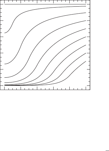
The minimum value for α occurs at the origin and takes the value

min

cosh x

. (4.31)

As x

increases, α

min

approaches zero; see Figure 4.2. For strong ﬁelds, and hence large

, we ﬁnd the asymptotic behavior

min

∼ exp(−x

). (4.32)

This relation is responsible for the collapse of the lapse, which we can see as follows: Sup-

pose we guess that as the maximal foliation proceeds, the interior ﬁeld-strength parameter

increases linearly with time t according to

= t/τ

+ constant, (4.33)

where τ

is some constant. We then would expect that at late times the minimum lapse will

decay as

min

∼ exp(−t/τ

). (4.34)

We might also guess that the e-folding time constant τ

would be comparable to M,

the mass of the source. In fact, such late-time exponential decay of the lapse has been

found in numerous numerical simulations employing maximal slicing.

For the dynamic

See, e.g., Smarr and York (1978a); Evans (1984); Petrich et al. (1985).

110 Chapter 4 Choosing coordinates: the lapse and shift

0.2

0.4

0.6

0.8

= 0

= 8

6810

Figure 4.2 The lapse α as a function of dimensionless radius x for select values of the parameter x

, plotted

according to the analytic model. The parameter x

varies between x

= 0(topcurve,α = 1) and x

= 8 (bottom

curve) in increments of unity. The “collapse of the lapse” is evident in the strong-ﬁeld region. [After Smarr and

Yo r k (1978a).]

maximally-sliced Schwarzschild spacetime discussed above and derived in Chapter 8.1,it

can be shown analytically

that the e-folding time is given by τ

= 3

√

6/4M ∼ 1.837M,

which is very close to the value 1.82 inferred from some of the earliest numerical calcula-

tions.

Proﬁles of the lapse for the exact solution are shown in Figure 8.4.

While many of its geometric properties are very desirable, maximal slicing also has some

computational disadvantages. The conditions (4.12)–(4.14) are spatial elliptic equations for

the lapse function α. Even though they are linear, such equations are often costly to invert

numerically in two and three dimensions. Since maximal slicing is only a coordinate gauge

condition, truly physical results extracted from a simulation should not be affected at all if

the maximal slicing condition is modiﬁed, or if the condition is satisﬁed only approximately.

This realization suggests that, instead of solving an elliptic equation, one could convert

that equation into a parabolic equation, which is much faster to solve numerically.

fact, one way of solving an elliptic equation, called “relaxation”, is to introduce a time

variable, recast the equation as a parabolic equation, and look for steady-state solutions.

An evolution that adopts an “approximate” maximal slicing condition presumably will

generate data that satisfy condition (4.10) only approximately. Suppose that during the

course of the evolution the data give rise to nonzero values of the mean curvature, K ,in

violation of condition (4.10). Maintaining the condition ∂

K = 0 after this occurs would

allow K to remain nonzero, which would not be consistent with maximal slicing. It would

Petrich et al. (1985); Beig and

O Murchadha (1998).

Smarr and York (1978a).

Balakrishna et al. (1996); Shibata (1999a).

See Chapter 6, where we discuss the classiﬁcation of partial differential equations, as well as computational strategies

for solving them.