Baumgarte T., Shapiro S. Numerical Relativity. Solving Einstein’s Equations on the Computer
Подождите немного. Документ загружается.


5.2 Hydrodynamics 131
Implementing an HRSC scheme to solve equation (5.26) then begins by calculating
the primitive variables
P on each cell interface (the “reconstruction step”). At most grid
points, the computed value of the primitive variable takes into account the variation of the
variable at the nearest points to the interface to high order in the adopted grid spacing.
When a discontinuity is identified at the interface (as in the case of a shock) by a “slope-
limiter” that looks for changes in the nearby slopes of variables, the order is reduced.
Next, the reconstructed data are used as initial data for a local Riemann problem (the
“Riemann solver step”). The net flux
F
i
at each cell interface is given by the solution to
this Riemann problem. Exact Riemann solvers require knowledge of the eigenvectors of
the system, while approximate Riemann solvers do not. The later, which provide simpler
HRSC schemes and are based on solving dispersion relations for the wave speeds in
the fluid, are often adequate.
11
Once the flux is employed to compute the conservative
variables
U at the new time step, these values are used to recover the primitive variables
P on the new time level (the “recovery step”). This may not be trivial because, while
the functional relations
U(P) are analytic, the inverse relations P(U) are usually not
and must be solved numerically. The whole process is then repeated for the next time
step.
We now catalog the source terms ρ, S
i
, S
ij
and S in terms of the primitive fluid variables
for a perfect gas. Substituting the fluid stress-energy tensor (5.4) into equations (5.1)–(5.2)
yields the fluid contributions to the source terms:
ρ
fluid
= ρ
0
hW
2
− P, (5.33)
S
fluid
i
= ρ
0
hWu
i
, (5.34)
S
fluid
ij
= Pγ
ij
+
S
fluid
i
S
fluid
j
ρ
0
hW
2
, (5.35)
S
fluid
= 3P + ρ
0
h(W
2
− 1). (5.36)
We insert the superscript “fluid” to remind us that the contribution from the perfect fluid
must be added to the contributions from all other nongravitational sources of energy-
momentum.
Smoothed particle hydrodynamics (SPH) schemes
Smooth particle hydrodynamics, or SPH, provides yet another way of treating a relativis-
tic fluid. The SPH method was originally introduced by Lucy (1977)andGingold and
Monaghan (1977) to handle Newtonian fluids in 3 + 1 dimensions. Most of the early
11
One of the simplest shock-capturing schemes that does not require knowledge of the eigenvectors is the HLL scheme
(Harten et al., 1983), which has been shown to perform with an accuracy comparable to more sophisticated Riemann
solvers in shock tube problems when coupled to a high-order reconstruction method like PPM (“piecewise parabolic
method”; Colella and Woodward (1984)).

132 Chapter 5 Matter sources
applications involved Newtonian stellar hydrodynamics. SPH was later adapted to treat
fully relativistic fluids, particularly in the context of relativistic core collapse, binary neu-
tron star mergers and binary black hole–neutron star mergers.
12
It has also been useful in
cosmology simulations of structure formation, where fluid baryonic matter and collision-
less “dark” matter must be evolved simultaneously.
SPH is a Lagrangian method that follows the behavior of fluid elements, represented
by a large sample of particles. The “forces” that govern the motion of the particles are
constructed from the equations of hydrodynamics. At any time, the positions of the particles
are assumed to be distributed in proportion to the fluid rest-mass density. Given a finite
distribution of particles, the density is determined statistically by introducing a “smoothing
kernel” in a Monte Carlo integral over the distribution. Pressure-gradient forces are also
calculated by kernel estimation, using the particle positions, rather than by direct evaluation
(e.g., finite-differencing) of the hydrodynamic equations.
The Lagrangian formulation employed in SPH introduces a Lagrangian time deriva-
tive d/dt in the fundamental hydrodynamic equations (5.12)–(5.14). The Lagrangian time
derivative follows changes in the properties of a given fluid element along its worldline and
is related to the Eulerian time derivative ∂
t
that measures changes at a fixed point in space
according to d/dt = ∂
t
+ v
j
∂
j
, where the fluid velocity v
j
is given by equation (5.23).
Substituting this Lagrangian time derivative in equation (5.12) gives the Lagrangian
continuity equation,
dρ
∗
dt
+ ρ
∗
∂
j
v
j
= 0, (5.37)
where ρ
∗
≡ γ
1/2
D ≡ αu
t
γ
1/2
ρ
0
.
13
This conservative form of the continuity equation
allows us to define a fixed set of particles, each of which is labeled by subscript “a”
and has a constant rest-mass m
a
. Each particle has an instantaneous position x
j
a
that moves
according to dx
j
a
/dt = v
j
a
. For each particle we define a “smoothing length” h
a
,which
represents the physical size of the particle. Thus, a particle does not have a delta-function
density profile, but instead represents a spherically symmetric density distribution of finite
radius (with typical radius =2h
a
) centered at the particle position. The density at each
particle is then determined as a locally weighted average by summing over all the particles
residing within this radius:
(
ρ
∗
)
a
=
b
m
b
W
ab
. (5.38)
Here W
ab
is a smoothing (or interpolation) kernel. It can be calculated for a pair of particles
as a function of r
ab
= (x
2
ab
+ y
2
ab
+ z
2
ab
)
1/2
, the coordinate distance from particle a to its
neighbor b,andh
a
. A second-order differentiable form often used for W was introduced
12
See Chapters 16 and 17 for details and references.
13
This density variable should not be confused with ρ
∗
defined below equation (5.5).

5.2 Hydrodynamics 133
by Monaghan and Lattanzio (1985) and is given by
W (r, h) =
1
πh
3
1 −
3
2
r
h
2
+
3
4
r
h
3
, 0 ≤
r
h
< 1,
1
4
$
2 −
r
h
%
3
, 1 ≤
r
h
< 2,
0,
r
h
≥ 2.
(5.39)
Note that W is normalized so that when integrated over all space,
W (r, h)4πr
2
dr = 1.
Tracking a fixed number of particles in a simulation and evaluating their density according
to equation (5.38) is equivalent to solving the continuity equation.
Exercise 5.9 Many of the applications of SPH in general relativity assume confor-
mally flat spacetimes, for which the metric is restricted to be of the form
ds
2
=−α
2
dt
2
+ ψ
4
η
ij
(dx
i
+ β
i
dt)(dx
j
+ β
j
dt). (5.40)
We have already encountered conformal flatness in Chapter 3.1.2, and will discuss
this approximation and its domain of validity in the context of dynamical simulations
in greater detail in Chapters 16.2 and 17.2.1.
Here we will adopt this metric, together with a -law EOS, and assemble
the remaining relativistic Lagrangian hydrodynamic equations used in many SPH
applications.
(a) Show that the Euler equation can be written in Lagrangian form as
d
˜
u
i
dt
=−
αψ
6
ρ
∗
∂
i
P − αhu
0
∂
i
α +
˜
u
j
∂
i
β
j
+
2hα(γ
2
n
− 1)
γ
n
ψ
∂
i
ψ, (5.41)
where the specific momentum is defined by
˜
u
i
≡ hu
i
. (5.42)
(b) Show that the energy equation can be written in Lagrangian form as
de
∗
dt
+ e
∗
∂
i
v
i
= 0, (5.43)
where e
∗
≡ γ
1/2
E ≡ αu
t
ψ
6
(ρ
0
)
1/
. Note that in the absence of shocks, the adia-
batic energy equation can be replaced by the polytropic equation (5.18).
The pressure gradient appearing the Lagrangian Euler equation (see, e.g., exercise 5.9)
is calculated according to
1
(ρ
∗
)
a
∂
i
P
a
=−
b
m
b
P
b
(ρ
∗
)
2
b
+
P
a
(ρ
∗
)
2
a
∂
i
W
ab
. (5.44)
Other terms depend on the metric functions and their derivatives.
14
Artificial viscosity can
be incorporated in a relativistic SPH scheme to handle shocks.
15
14
Recipes for choosing the smoothing kernels and lengths and for evaluating the full set of relativistic SPH equations in
conformally flat spacetimes are given in, e.g., Oechslin et al. (2002)andFaber et al. (2004), and references therein.
15
Siegler and Riffert (2000); Oechslin et al. (2002).
134 Chapter 5 Matter sources
SPH is perhaps the simplest hydrodynamics scheme to implement for simulating multi-
dimensional fluid systems. It is also well suited for tracing the Lagrangian flow of matter,
which is particularly convenient when different fluid species are present and mix. However,
a large number of particles are required, and their positions must be carefully tracked, in
order to minimize numerical errors. Low-resolution SPH calculations tend to be noisy,
and this noise can lead to spurious diffusion of SPH particles and spurious viscosity,
independent of any real physical mixing and physical viscosity.
16
Rankine–Hugoniot conditions
Shock waves pose the most serious challenge for any numerical hydrodynamical scheme.
The ability to resolve the sharp discontinuities in the fluid parameters associated with a
shock is typically what distinguishes one code from the next. This fact motivates a brief
discussion here of a few of the key equations that relate the fluid variables across a shock
front.
17
The Rankine–Hugoniot junction conditions across a relativistic shock discontinuity
can be derived easily from the fundamental hydrodynamic equations (5.6) and (5.7).
Integrating ∇
b
T
ab
and ∇
a
(ρ
0
u
a
) over a “pill box” centered on the shock front, and using
Gauss’ theorem, gives the junction conditions,
[ρ
0
u
a
ˆ
z
a
] = 0, (5.45)
and
[T
ab
ˆ
z
b
] = 0, (5.46)
where
ˆ
z
a
is the spacelike normal vector to the front. Here the bracket denotes the difference
between quantities on the two sides of the shock front; [V ] ≡ V
+
− V
−
, where “+” labels
the front side of the shock (the side upstream) and “−” labels the back side (the side
downstream). The first condition can be written as
F ≡ ρ
+
0
u
a
+
ˆ
z
a
= ρ
−
0
u
a
−
ˆ
z
a
, (5.47)
where F is the conserved flux of rest-mass across the front. Using definition (5.4)inthe
second condition allows us to write
F(h
+
u
a
+
− h
−
u
a
−
) =
ˆ
z
a
(P
−
− P
+
). (5.48)
16
For a study of spurious transport effects in Newtonian SPH calculations, and other potential difficulties, see Hernquist
(1993)andLombardi et al. (1999), and references therein.
17
For a detailed treatment of relativistic shocks, see, e.g., Taub (1948); Lichnerowicz (1967); Landau and Lifshitz (1959);
Novikov and Thorne (1973). The discussion here is patterned after Evans (1984).
5.2 Hydrodynamics 135
Contracting equation (5.48) alternately with u
+
a
and u
−
a
, and taking the difference of the
two equations, yields the relativistic Rankine–Hugoniot relation,
h
2
+
− h
2
−
=
h
+
ρ
+
0
+
h
−
ρ
−
0
(P
+
− P
−
). (5.49)
Exercise 5.10 Take the nonrelativistic limit of equation (5.49) to get the standard
Rankine–Hugoniot relation
+
−
−
=
P
+
+ P
−
2ρ
+
0
ρ
−
0
(ρ
+
0
− ρ
−
0
). (5.50)
To determine the “jump” in rest-mass density across a shock front it is useful to cast
equation (5.49) in nondimensional form,
H
2
− 1 = δ
2
(y − 1)
H
η
+ 1
, (5.51)
where we have introduced the nondimensional variables H = h
+
/ h
−
, y = P
+
/P
−
,η =
ρ
+
0
/ρ
−
0
and δ
2
= p
−
/(ρ
−
0
h
−
). The ratio H can be eliminated from the above equation by
introducing an EOS. Employing our -law EOS (5.17) and defining q ≡ 1/ h
−
gives a
quadratic equation for the density ratio η, parametrized by q, and to be solved as a function
of the pressure ratio y:
[
y( −1) + (q + 1)
]
η
2
− q
[
y( +1) + ( − 1)
]
η − (1 − q)y(y + − 1) = 0.
(5.52)
The parameter q measures the degree to which the flow is relativistic: q → 1 for nonrel-
ativistic (NR) flow, while q → 0 for extremely relativistic (ER) flow. Taking the nonrela-
tivistic limit of equation (5.52)gives
η =
y( +1) + ( − 1)
y( −1) + ( + 1)
. (5.53)
The parameter y measures the strength of the shock: y →∞for strong shocks, while
y → 1 for weak shocks (acoustic waves). Taking the strong shock limit of equation (5.53)
gives the familiar Newtonian result for the maximum compression behind a strong shock,
η →
+ 1
− 1
(strong NR shock). (5.54)
For an extremely relativistic shock, equation (5.52)gives
η =
&
y(y + − 1)
y( −1) + 1
'
1/2
. (5.55)
By contrast with the Newtonian result, the maximum compression behind a strong rela-
tivistic shock has no upper limit, but increases steadily with y according to
η →
&
y
− 1
'
1/2
(strong ER shock). (5.56)
136 Chapter 5 Matter sources
1
0.8
0.6
0.4
0.2
0
0–1 –0.5 0.5 1
x
V
P/200
r
0
/10
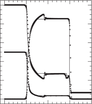
Figure 5.1 A one-dimensional relativistic Riemann shock tube test for an ideal fluid with an adiabatic index
= 2. The plot shows the numerically evolved rest density ρ
0
(triangles), pressure P (squares), and velocity v
(crosses) at t = 0.5. The analytic values are indicated by solid curves. This calculation used the Wilson scheme
with artificial viscosity P
vis
= C
vis
A(δv)
2
, A = γ
1/2
D, δv = 2∂
k
v
k
x ,andC
vis
= 1. [From Duez et al.
(2003).]
Not surprisingly, the strongest and most relativistic shocks pose the most stringent test for
a numerical hydrodynamics code, as the discontinuities are steepest in this regime.
Tests
Testing a code designed to handle relativistic hydrodynamics is an essential and nontrivial
phase of code construction. Convergence tests often serve as the initial step in code
validation, providing the first line of defense against coding errors and bugs, including
simple typos.
18
To fully calibrate the reliability and robustness of a code it is necessary
to run a suite of test-bed problems, the solutions to which are known. One might start
by fixing the spacetime to be Minkowski, which allows the fluid sector of the code to
be tested in special relativity. Performing a relativistic Riemann shock tube problem is
particularly instructive in this case. The problem provides a “pure” hydrodynamics test,
since no complications from the numerical treatment of the gravitational field equations
can arise. It also provides a rather strenuous test, since a shock wave reflects the full
nonlinear character of the hydrodynamic equations.
We illustrate such a test in Figure 5.1 for a simple one-dimensional shock tube. We
consider an ideal fluid and adopt a -law EOS with = 2. At t = 0wesetv
x
= 0
everywhere while for x < 0wesetρ
0
= 10, P = 100 and for x > 0wesetρ
0
= 1,
18
See Chapter 6.4.
5.2 Hydrodynamics 137
P = 1. The solution is evolved with a second-order, finite difference scheme based on
the Wilson method using artificial viscosity. Here a grid of 400 points is employed over
a domain x ∈ (−1, 1). The shock is modeled rather well, apart from an “overshoot” in
quantities at the rarefaction (i.e., low density expansion) front. It has been shown
19
that in
finite difference schemes using artificial viscosity, such an overshoot arises in numerical
solutions even when the grid spacing goes to zero. This limitation of artificial viscosity
methods is particularly serious when strong shocks are present; HRSC techniques help
overcome this difficulty.
Exercise 5.11 Show that the results plotted in Figure 5.1 are consistent with equa-
tion (5.55).
In curved spacetime, the set of known, analytic solutions to the equations of relativis-
tic hydrodynamics is not large, particularly for dynamical spacetimes. Holding a stable,
static, spherical star constructed from the OV hydrostatic equilibrium equations in stable
equilibrium (see Chapter 1.3) provides one simple test. Holding a stable, stationary, rotat-
ing star constructed from the stationary equilibrium equations in stable equilibrium (see
Chapter 14.1) constitutes a more challenging test, particularly if it is differentially rotat-
ing and therefore subject to spurious redistribution of angular momentum by numerical
viscosity. The analytic Oppenheimer–Snyder solution
20
for the collapse of a spherical,
homogeneous ball of dust from rest at finite radius provides an analytic dynamical space-
time for testing the ability of a code to handle catastrophic collapse of a fluid to a black
hole. The interior solution is analytic in geodesic slicing and comoving radial coordinates
and must be transformed numerically in order to compare with numerical integrations
performed in different time slicings and/or spatial coordinates.
21
Alternatively, the ana-
lytic solution, which is easily expressed in closed-Friedmann form in the matter interior
and Schwarzschild in the vacuum exterior, can be employed to construct various scalar
invariants (e.g., areal radii R(τ ) of Lagrangian fluid elements as functions of proper time
τ in the interior, and Riemann curvature invariants in the exterior) that can readily test a
dynamical simulation performed in an arbitrary gauge.
During any numerical simulation it is useful to monitor quantities whose values ought
to be conserved. For example, the global conserved quantities discussed in Section 3.5
provide useful checks. The total rest mass of the system M
0
must be conserved, provided
we account for any rest mass that leaves the computational domain. The ADM mass
M
ADM
, the total linear momentum P
i
ADM
and angular momentum J
i
ADM
are also conserved,
provided we account for net losses carried off by any matter and gravitational radiation
that leave the computational domain. Other hydrodynamic quantities are useful to monitor
in special cases. For example, the relativistic Bernoulli integral is conserved along flow
19
Norman and Winkler (1983).
20
See Chapter 1.4.
21
See Petrich et al. (1985, 1986), who construct the Oppenheimer–Snyder solution for both maximal and polar time
slicing and isotropic radial coordinates.

138 Chapter 5 Matter sources
lines for adiabatic, stationary flow with 4-velocity u
a
in a stationary gravitational field:
22
hu
t
= constant (along flow lines). (5.57)
For a uniformly rotating, stationary, perfect fluid star, we have
h
u
t
= constant, (5.58)
where the constant holds everywhere inside the fluid. This result is satisfied whenever the
spacetime has two Killing vectors, ξ
a
(t)
= (∂/∂t)
a
and ξ
a
(φ)
= (∂/∂φ)
a
, to reflect stationarity
and axisymmetry.
23
The Kelvin–Helmholtz theorem states that the relativistic circulation,
C(c) =
(
c
hu
a
λ
a
dσ, (5.59)
is conserved for isentropic flow along an arbitrary closed “fluid” contour c.
24
Here σ is a
Lagrangian parameter which labels fluid elements on the contour c,andλ
a
is the tangent
vector to the contour [i.e., λ
a
= (∂/∂σ)
a
]. Conservation of C can be verified by computing
d
dτ
C(c) =
(
c
dσ u
b
∇
b
(hu
a
λ
a
)
=
(
c
dσ
λ
a
u
b
∇
b
(hu
a
) + (hu
a
)u
b
∇
b
λ
a
=
(
c
dσ [λ
a
u
b
∇
b
(hu
a
) + (hu
a
)λ
b
∇
b
u
a
]
=−
(
c
dσλ
a
∇
a
h
= 0. (5.60)
Here, to derive the third line from the second line, we use the fact that u
a
= (∂/∂τ)
a
and
λ
a
are coordinate basis vectors, and thus commute according to
u
b
∇
b
λ
a
= λ
b
∇
b
u
a
. (5.61)
We also have used u
a
u
a
=−1 and the Euler equation for isentropic flow in the form
u
b
∇
b
(hu
a
) =−∇
a
h (5.62)
to obtain the fourth line. Note that it is the derivative of
C(c) with respect to the proper time
τ that vanishes, so that the circulation has to be evaluated on hypersurfaces of constant
proper time as opposed to constant coordinate time.
22
Lightman et al. (1975), Problem 14.7, p. 83
23
ibid., Problem 16.17, p. 95. Actually, the result holds even when ξ
a
(t)
and ξ
a
(φ)
are not Killing vectors separately
but combine to form a helical Killing vector ξ
a
hel
= ξ
a
(t)
+ ξ
a
(φ)
,where is the angular velocity of the fluid; see
Chapter 15.2 and equation (15.46) for a proof.
24
See Landau and Lifshitz (1959); Taub (1959); Evans (1984); Saijo et al. (2001).

5.2 Hydrodynamics 139
Exercise 5.12 Show that for general (e.g., nonisentropic) flows, the Euler equation
is
u
b
∇
b
(hu
a
) =−
1
ρ
0
∇
a
P =−∇
a
h + T ∇
a
s, (5.63)
and the circulation changes according to
d
dτ
C(c) =−
(
c
dσλ
a
1
ρ
0
∇
a
P =
(
c
dσλ
a
T ∇
a
s. (5.64)
Comment on the implications of this result for a shock.
5.2.2 Imperfect gases
There are many important astrophysical applications that involve imperfect gases char-
acterized by viscosity, conductivity and (or) radiation. For example, viscosity can drive
nonaxisymmetric instabilities in rotating stars, while radiation can lead to the cooling and
contraction of stars. However, most of the numerical work to date in relativistic hydrody-
namics has focused on perfect fluid sources.
25
This emphasis is physically reasonable for
tracking evolution on dynamical (e.g., free-fall) time scales, but is not adequate for fol-
lowing evolution on secular (e.g., viscous, conduction or radiative) time scales, which are
typically much longer. As the field of numerical relativity matures, exploration of secular
behavior over many dynamical timescales is likely to accelerate. For this reason, we shall
now briefly summarize additional contributions to the stress-energy tensor arising from
some of these nonideal effects.
Viscosity
The contribution of viscosity to the stress-energy tensor is
26
T
ab
visc
=−2ησ
ab
− ζθP
ab
(5.65)
where η ≥ 0 is the coefficient of dynamic, or shear, viscosity, ζ ≥ 0 is the coefficient of
bulk viscosity and σ
ab
,θ, P
ab
are the shear, expansion and projection tensor of the fluid:
θ =∇
a
u
a
, (5.66)
P
ab
= g
ab
+ u
a
u
b
, (5.67)
σ
ab
=
1
2
P
ac
∇
c
u
b
+ P
bc
∇
c
u
a
−
1
3
θ P
ab
. (5.68)
Exercise 5.13 Show that in the presence of viscosity, the energy (entropy) equa-
tion (5.19) becomes
∂
t
(γ
1/2
E
∗
) + ∂
j
(γ
1/2
E
∗
v
j
) =
αγ
1/2
E
∗
W
(1−)
2ησ
ab
σ
ab
+ ζθ
2
. (5.69)
25
But see, e.g., Duez et al. (2004) and Chapter 14.2.4 for relativistic hydrodynamical simulations with viscosity.
26
See Misner et al. (1973), Section 22.3
140 Chapter 5 Matter sources
Thus conclude by comparing with equation (5.21) that viscosity generates entropy
at a rate
ρ
0
T
ds
dτ
=
2ησ
ab
σ
ab
+ ζθ
2
. (5.70)
Exercise 5.14 Show that in the presence of viscosity, the momentum equation (5.14)
becomes
∂
t
(γ
1/2
S
i
) + ∂
j
(γ
1/2
S
i
v
j
) =
− αγ
1/2
∂
i
P +
S
a
S
b
2αS
t
∂
i
g
ab
+ αγ
1/2
ησ
ab
∂
i
g
ab
+ 2∂
a
αγ
1/2
ησ
ib
g
ab
+
1
2
αγ
1/2
ζθP
ab
∂
i
g
ab
+ ∂
a
αγ
1/2
ζθP
ib
g
ab
. (5.71)
The presence of time derivatives of u
a
in σ
ab
and the time derivative of σ
ab
on the
right hand side of the nonconservative, relativistic Navier–Stokes equations (5.69)and
(5.71) require subtle handling. Since viscosity is usually a small perturbation on the
dynamical flow, it is often sufficient to split off the viscous terms and integrate them
separately (“operator splitting”) in a lower-order, but convergent, scheme.
27
When recast
in conservative form as in equation (5.26), the dynamical equations for the “conservative”
variables (
˜
D,
˜
S
j
, ˜τ) appear unchanged when nonideal gas contributions are added to the
stress-energy tensor. However, the character of the equations is altered, as there now are
additional derivatives (including time derivatives) of the primitive variables that appear in
these variables and in their source terms. Once again, a lower-order scheme to handle these
perturbative terms is often adequate.
Heat and radiation diffusion
The contribution of heat flux (i.e., conduction) to the stress-energy tensor is
T
ab
heat
= u
a
q
b
+ u
b
q
a
, (5.72)
where the heat-flux 4-vector q
a
is given by
q
a
=−λ
th
P
ab
(
∇
b
T + Ta
b
)
. (5.73)
In equation (5.73), T is the temperature, a
a
= u
b
∇
b
u
a
is the fluid 4-acceleration, and λ
th
is the coefficient of thermal conduction.
A useful application of the thermal conduction formalism is heat transport via thermal
radiation (e.g., photons or neutrinos) treated in the diffusion approximation, for which
λ
th
=
4
3
b
R
T
3
¯χ
. (5.74)
27
See Duez et al. (2004) and Chapter 14.2.4 for such an approach.