Birge J.R., Louveaux F. Introduction to Stochastic Programming

Подождите немного. Документ загружается.

74 2 Uncertainty and Modeling Issues

2.8 Modeling Exercise

In this section, we propose a modeling exercise and comment on a number of pos-

sible answers.

a. Presentation

Consider a production or assembly problem. It consists of producing two products,

say A and B . They are obtained by assembling two components, say C1andC2,

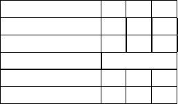
in ﬁxed quantities. The following table shows the components usage for the two

products:

Components usage A B

C1 6 10

C2 8 5

Components are produced within the plant. Material (and / or operating) costs for

C1andC2are0.4and1.2 , respectively. The level of production, or capacity,

is related to the work-force and the equipment. Each unit of capacity costs 150

and 180 and can produce batches of 60 and 90 components, respectively for C1

and C2 . Current capacity level is (40,20) batches and cannot be decreased. The

total number of batches must not exceed 120. An integer number of batches is not

requested here.

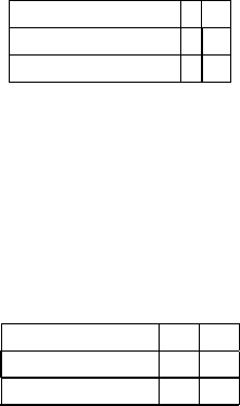
In the deterministic case, the demands and unit selling prices are certain and are

as follows:

A B

Demand 500 200

Unit selling price 50 60

Unmet demand results in lost sales. This does does not imply any additional penalty.

1. Select adequate units for each data. Formulate and solve the deterministic

problem.

Then, consider a number of stochastic variants. For the sake of comparison, in all

cases, the random variables have expectations which are the corresponding deter-

ministic values.

2.8 Modeling Exercise 75

2. Stochastic prices (known demand).

The selling prices of A and B are described by a random vector, say ζ

=(ζ

,ζ

) .

The rest of the data is unchanged. Formulate a recourse model in the following

cases:

(a) ζ

takes on the values (54,56) , (50,60) ,and (46,64) with probability 0.3,

0.4and0.3 respectively.

(b) ζ

takes on the values (46,50,54) with probability 0.3, 0.4and0.3; ζ

takes on the values (56,60, 64) with probability 0.3, 0.4and0.3; ζ

and ζ

are independent.

has a continuous uniform distribution in the range [46, 54] ; ζ

has a con-

tinuous uniform distribution in the range [56,64] ; ζ

and ζ

are independent.

(d) ζ

takes on the values (70,50) , (50,60) , (30, 70) with probability 0.3, 0.4

and 0.3.

(e) ζ

takes on the values (30,50,70) with probability 0.3, 0.4and0.3; ζ

takes on the values (50,60, 70) with probability 0.3, 0.4and0.3; ζ

and ζ

are independent.

3. Stochastic demands (known prices).

The demand levels of A and B are described by a random vector, say η

(η

,η

) . The rest of the data is as in the deterministic model.

(a) Formulate and solve a recourse model when η

takes on the values (400,100) ,

(500,200) , (600, 300) with probability 0.3, 0.4and0.3.

(b) Assume η

and η

are independent random variables with normal distribu-

tions, η

∼ N(500,6000) and η

∼ N(200,12000) . Find the optimal solution

of the recourse problem if the production of A and B is decided in the ﬁrst-

stage and there is no restriction at all on the number of batches of C1andC2.

batches must not exceed 120 . Also ensure that the probability that the demand

of B is covered must be larger than 80%.

4. Stochastic prices and demands.

Demands and prices are described by three scenarios S1, S2andS3 , as follows.

Demand level S1 S2 S3

A 700 500 300

B 100 200 300

Unit selling price

A 45 50 55

B 70 60 50

76 2 Uncertainty and Modeling Issues

Formulate and solve a recourse model assuming the three scenarios have probability

0.3, 0.4and 0.3 respectively.

5. Obtain EVPI and VSS for some relevant cases among these alternatives.

b. Discussion of solutions

1. Choice of units and deterministic model.

Units are as follows. First, deﬁne the unit of time. We may assume here data are

given per day for example. Then, demand is the number of units of A and B per

day. Selling prices are given as $ per unit of A and B . The level of production

is given by the number of batches (of 60 C1 and 90 C2 ) per day. Capacity cost

must include work-force cost, operating costs, and depreciation per day. Material

costs are $ per component. The distinction among these costs is important for the

stochastic model.

There is more than one formulation for the deterministic problem. The following

formulation (M1) is useful in view of later stochastic models. Let

• x

= number of batches of C1 available for production;

• x

= number of batches of C2 available for production;

• x

= number of units of A produced and sold per day;

• x

= number of units of B produced and sold per day.

For batches of C1andC2 , the objective contains the daily capacity cost. For

products A and B , it contains the selling price minus the material costs. (Each

unit of A , e.g. has a selling price of $50. It requests 6 units of C

and 8 units

of C

for a total material cost of $12. The difference is the objective coefﬁcient

38 .) The ﬁrst two constraints state that the usage of components is smaller than

the availability. The third constraint is the upper limit on the number of batches.

Demand and capacity bounds follow.

(M1) z = max−150x

−180x

+ 38x

+ 50x

s. t. 6x

+ 10x

≤ 60x

+ 5x

≤ 90x

+ x

≤ 120,

40 ≤ x

, 20 ≤ x

, 0 ≤x

≤ 500 , 0 ≤x

≤ 200.

The optimal solution of (M1) is z = 5800 , x

= 220/3, x

= 140/3, x

= 400 ,

= 200 . Product B is at the maximum corresponding to its demand. All 120

batches of capacity are used. The rest of the solutions follow.

A shorter formulation (M2) is to deﬁne two variables:

• x

= number of units of A produced and sold per day;

• x

= number of units of B produced and sold per day.

2.8 Modeling Exercise 77

This formulation requires computing the margins of A and B . Each unit of A

obtains the selling price of $50. It requires 6 components C1 and 8 components C2

for a total material cost of $12. It also requires 6/60 batches of capacity for C1and

8/90 batches for C2 at a cost of $31. The net margin for A is thus $7 per unit. Sim-

ilarly, the net margin for B is $15 per unit. Note that this calculation of the margins

of A and B is only valid if there is no unused capacity or unsold product, which

is not always the case in a stochastic model. The ﬁrst two constraints correspond to

maintaining at least the existing capacity levels of 40 and 20 respectively. The third

constraint corresponds to a maximal capacity level of 120 (each unit of A requires

6/60 of C1and8/90 of C2 , or 17/90 capacity units; each unit of B requires

10/60 of C1and5/90 of C2or20/90 capacity units). The model also includes

the demand constraints and reads as follows:

(M2) z = max7x

+ 15x

s. t. 6x

+ 10x

≥ 2400,

+ 5x

≥ 1800,

17x

+ 20x

≤ 10800,

0 ≤ x

≤ 500 , 0 ≤x

≤ 200.

This model has the same optimal solution, z = 5800 , x

= 400 , x

= 200 , as

previously. It is clear in (M2) that the margin of B is larger than that of A . Thus,

product B is at the maximum corresponding to its demand. Product A is then

reduced from the limit of 120 batches of capacity. The number of batches for C1

and C2 can be computed from the production of A and B , and are equal to 220/3

and 140/3 , respectively.

2. Stochastic prices.

The essential modeling question concerns the timing of the decisions. Typically, the

capacity decisions are made in the long run. They are ﬁrst-stage decisions. Sales oc-

cur when the price is known. They are always second-stage decisions. Depending on

the ﬂexibility of the production process, the decision on the quantity to be produced

may be ﬁrst- or second-stage. We may thus distinguish between two formulations:

production is ﬁrst-stage (M3) or second-stage (M4).

2.1. Production is ﬁrst-stage.

Let

• x

= number of batches of C1 available for production;

• x

= number of batches of C2 available for production;

• x

= number of units of A produced per day;

• x

= number of units of B produced per day;

• y

= number of units of A sold per day;

• y

= number of units of B sold per day;

78 2 Uncertainty and Modeling Issues

z = max−150x

−180x

−12x

−10x

+ E

(

) y

(

)+q

(

) y

(

))

s. t. 6x

+ 10x

≤ 60x

+ 5x

≤ 90x

+ x

≤ 120

(

) ≤x

, y

(

) ≤ x

40 ≤ x

, 20 ≤ x

, 0 ≤x

0 ≤ y

(

) ≤500, 0 ≤y

(

) ≤ 200,

where ξ

(

)=(q

(

),q

(

)) = ζ

(

) corresponds to the selling prices.

In practice, it is customary to use a simpliﬁed notation where the dependence of

y and ξ on

is not made explicit. This (abuse of) notation is used here.

(M3) z = max−150x

−180x

−12x

−10x

+ E

+ q

)

s. t. 6x

+ 10x

≤ 60x

+ 5x

≤ 90x

+ x

≤ 120,

≤ x

, y

≤ x

40 ≤ x

, 20 ≤ x

, 0 ≤x

0 ≤ y

≤ 500 , 0 ≤y

≤ 200,

where ξ

=(q

)=ζ

We now transform (M3) as in Section 2.4a. Assuming q

and q

are never

negative (a much needed assumption for the producer to survive), we obtain

(M3’) z = max−150x

−180x

−12x

−10x

min{x

,500}+ q

min{x

,200})

s. t. 6x

+ 10x

≤ 60x

+ 5x

≤ 90x

+ x

≤ 120,

40 ≤ x

, 20 ≤ x

, 0 ≤x

(M3”) z = max−150x

−180x

−12x

−10x

min{x

,500}+

min{x

,200}

s. t. 6x

+ 10x

≤ 60x

+ 5x

≤ 90x

+ x

≤ 120

40 ≤x

, 20 ≤ x

, 0 ≤x

where (

) is the expectation of ξ

As (

) is equal to the deterministic selling prices (50, 60) , it is easy to

show that (M3”) has the same optimal solution as the model (M1). This is true

for each of the considered cases (a) to (e). To put it another way, if production is

decided in the ﬁrst-stage, the stochastic model where only the selling prices are

2.8 Modeling Exercise 79

random can be replaced by a deterministic model with the random prices replaced

by their expectations.

2.2. Production is second-stage

Let x

and x

be as in (M3) and

• y

= number of units of A produced and sold per day;

• y

= number of units of B produced and sold per day.

(M4) z = max−150x

−180x

+ E

+ q

)

s. t. x

+ x

≤ 120,

+ 10y

≤ 60x

+ 5y

≤ 90x

40 ≤ x

, 20 ≤ x

, 0 ≤y

≤ 500 , 0 ≤y

≤ 200,

where ξ

=(q

)=ζ

−(12,10) corresponds to selling prices minus material

costs.

Before using formulation (M4), consider the deterministic formulation (M2). As

long as the margin of B is larger than the margin of A and the margin of A re-

mains positive, it is optimal to produce and sell 400 A and 200 B . If this holds for

all realizations of the selling prices, the same optimal solution is obtained for all re-

alizations of ζ . It is thus the optimal solution of the stochastic model. (This will be

elaborated in the comments after Proposition 5 of Chapter 4.) The expected margin

is simply E

(400ζ

+ 200ζ

−26,200) where 26,200 is the total of the material

and capacity costs for the daily production of 400 A and 200 B .As (ζ

,ζ

) has

expectation (50,60) as in the deterministic model, the expected margin is again the

same as in the deterministic model. This situation occurs in cases (a), (b) and (c)

of this exercise: the margin of A is ζ

−43 , the margin of B is ζ

−45 and the

relation ζ

−45 ≥ ζ

−43 ≥ 0 holds.

If at some point, the margin of A becomes negative or exceeds that of B ,then

(M4) is a truly stochastic model. For cases (d) and (e), there are values of the selling

prices where the margin of A exceeds that of B . The stochastic model (M4) has to

be solved.

In case (d), ζ

takes on the values (70,50) , (50,60) , (30,70) with probability

0.3, 0.4and0.3 , respectively. First-stage optimal capacity decisions are (x

(69.167,50.833) . Second-stage optimal production and sale decisions (x

) are

(500,115) , (500, 115) and (358.333, 200) for the three possible scenarios. The

optimal objective value is z = 5990 .

In case (e), the two random variables ζ

and ζ

are independent, taking three

different values each. Thus, the second-stage must consider 9 realizations. The op-

timal solution is the same as in the deterministic case: ﬁrst-stage decisions are

)=(73.333,46.667) , second-stage decisions are (x

)=(400,200) , with

objective value z = 5800 .

80 2 Uncertainty and Modeling Issues

3. Stochastic demands.

(a) As in Question 2, the ﬁrst modeling question is the timing of the decisions.

Capacity decisions are made in the long run and are ﬁrst-stage decisions. Sales occur

when price is known and are second-stage. The decisions on the quantities to be

produced may be ﬁrst- or second-stage.

(a.1) Production is ﬁrst-stage.

If production is ﬁrst-stage, lost sales occur when demand exceeds production. What

happens when production exceeds demand is problem dependent. In some situa-

tions, excess production may be held in inventory. This would be the case when

the randomness represents day-to-day variations in demand. Then excess produc-

tion is used later to compensate for possible lost sales. Randomness only results in

inventory costs. On the other hand, for products such as perishable goods, produc-

tion is lost ( C1andC2 could be ﬂour and eggs, A and B could be bread and

pastry, e.g.) and lost sales cannot be compensated. The same is true when the ran-

domness describes a set of scenarios of which only one is realized. The scenarios

could represent the uncertainty about the success of a new product. If a product is

not successful, extra production is lost. If it is very successful, sales are lost to com-

petitors if the production level is insufﬁcient. Or, alternative actions are needed such

as subcontracting or overtime.

We now present a formulation (M5) corresponding to a scenario situation (excess

production is lost, lost sales are not compensated). The decision variables are the

same as in (M3).

(M5) z = max−150x

−180x

−12x

−10x

+ E

(50y

+ 60y

)

s. t. 6x

+ 10x

≤ 60x

+ 5x

≤ 90x

+ x

≤ 120,

≤ x

, y

≤ x

40 ≤ x

, 20 ≤ x

, 0 ≤x

0 ≤ y

≤ d

, 0 ≤y

≤ d

where ξ

=(d

)=η

correspond to the demand level.

The ﬁrst-stage optimal capacity decisions are (x

)=(56.667,41.111) .The

second-stage optimal production and sale decisions (x

) are

(400,100) in the three possible scenarios. The optimal objective value is z = 4300 .

Observe that the production is set to meet the lowest possible demand.

2.8 Modeling Exercise 81

(a.2) Production is second-stage.

If production is second-stage, lost sales occur when the available production capac-

ities are insufﬁcient to cover the demand. Excess production does not occur as the

level of production can be adjusted to the downside. The decision variables are the

same as in (M4). Formulation (M6) reads as follows:

(M6) z = max−150x

−180x

+ E

(38y

+ 50y

)

s. t. x

+ x

≤ 120,

+ 10y

≤ 60x

+ 5y

≤ 90x

40 ≤ x

, 20 ≤ x

, 0 ≤y

≤ d

, 0 ≤y

≤ d

where ξ

=(d

)=η

corresponds to the demand level.

The ﬁrst-stage optimal capacity decisions are (x

)=(67.083,41.111) .The

second-stage optimal production and sale decisions (x

) are

(400,100) , (337.5, 200) and (337.5,200) for the three possible scenarios. The

optimal objective value is z = 4575 . Observe that the capacity limit of 120 batches

is not fully used.

(b) We consider a variant of formulation (M5) where the only constraints on x

and

are the components usage:

(M7) z = max−150x

−180x

−12x

−10x

+ E

(50min{x

}+ 60min{x

})

s. t. 6x

+ 10x

≤ 60x

+ 5x

≤ 90x

0 ≤ x

, 0 ≤x

where ξ

=(d

)=η

corresponds to the demand level.

Clearly, the two constraints are always tight. Replacing x

by (6x

+ 10x

)/60

and x

by (8x

+ 5x

)/90 , the model becomes

z = max{−43x

−45x

+ E

(50min{x

}

+ 60min{x

}) |0 ≤ x

, 0 ≤x

} ,

(M7’) z = max{−43x

+ 50E

min{x

,ξ

}−45x

+ 60E

min{x

,ξ

}|0 ≤x

, 0 ≤x

This optimization is separable in x

and x

. Both variables will be nonzero. So,

we are searching twice for the unconstrained minimum of an expression of the form

−ax+bQ(x) , with Q(x)=E

min{x,ξ} and ξ ∼N(

) . From Exercise 2.8.2,

we obtain that Q



(x)=1−F(x) .As Q



(x)=−f (x) , the second-order conditions

are satisﬁed. Thus the unconstrained minimum is obtained for Q



(x)=a/b ,i.e.

1 −F(x)=a/b .

Denote by F

(·) the cumulative distribution of ξ

, i = 1,2. For x

, the un-

constrained optimum satisﬁes 1 −F

)=43/50 , or F

)=0.14 . It corre-

sponds to a quantile q = −1.08 and a decision x

= 500 −1.08

√

6000 = 416.34 .

For x

,wehave 1− F

)=45/60 , or F

)=0.25 . It corresponds to a

82 2 Uncertainty and Modeling Issues

quartile q = −0.675 and a decision x

= 200 −0.675

√

12000 = 126.06 . For

the sake of comparison, we may compute x

=(6x

+ 10x

)/60 = 62.644 and

=(8x

+ 5x

)/90 = 44.011 . Also, using the closed form expression of Q(x) ,

(see again Exercise 2.8.2), one can obtain the optimal value of z .

than 80% is P(x

≥ ξ

) ≥ 0.8orF

) ≥ 0.8 . The 0.8 quantile is 0.84 . Thus,

) ≥ 0.8 is equivalent to (x

−

≥ 0.8,or x

≥ 200 + 0.84

√

12000 , or

≥ 292.02 .

The model to solve is:

(M8) z = max{−43x

+ 50E

min{x

,ξ

}−45x

+ 60E

min{x

,ξ

}|0 ≤ x

292.02 ≤ x

, 17x

+ 20x

≤10800},

where the constraint on the 120 batches has been transformed as in (M2).

By applying the Karush-Kuhn-Tucker conditions (see Review Section 2.11c.),

one can show that (x

)=(291.74,292.02) is the optimal solution.

4. Just as in the previous cases, there are two possible formulations as the produc-

tion decisions may be ﬁrst- or second-stage. Model (M9) corresponds to ﬁrst-stage

production while (M10) corresponds to second-stage production.

(M9) z = max−150x

−180x

−12x

−10x

+ E

+ q

)

s. t. 6x

+ 10x

≤ 60x

+ 5x

≤ 90x

+ x

≤ 120,

≤ x

, y

≤ x

40 ≤ x

, 20 ≤ x

, 0 ≤x

0 ≤ y

≤ d

, 0 ≤y

≤ d

where ξ

=(q

) , with q

and q

the selling prices and d

and d

the

demands jointly deﬁned in a scenario. Thus ξ

=(45,70,700,100),(50,60,500,200)

and (55,50,300, 300) with probability 0.3, 0.4,and 0.3 respectively. The opti-

mal solution is z = 3600 , (x

)=(46.667,32.222) with corresponding (x

(300,100) . The second-stage decisions are (y

)=(300,100) in all three sce-

narios. As the production cannot be adapted to the demand, the optimal solution is

to plan for the lowest demand and the expected margin is low.

(M10) z = max−150x

−180x

+ E

+ q

)

s. t. x

+ x

≤ 120

+ 10y

≤ 60x

+ 5y

≤ 90x

40 ≤ x

, 20 ≤ x

, 0 ≤y

≤ d

, 0 ≤y

≤ d

where ξ

=(q

) with q

and q

the selling prices minus the material

costs and d

and d

the demands. Thus, ξ

=(33, 60,700, 100) , (38,50, 500,200)

and (43,40,300,300) with probability 0.3, 0.4, and 0.3 . The optimal solu-

tion is z = 4048.75 , (x

)=(73.333,46.667) . The second-stage decisions are

)=(462.5, 100) , (400,200) and (300,260) in the three scenarios. While

2.8 Modeling Exercise 83

obtaining the optimal solution of (M10) with your favorite LP solver, you may ob-

serve that there is a high shadow price for the maximum number of batches.

Exercises

1. Consider Exercise 1 of Section 1.6.

(a) Show that this is a two-stage stochastic program with ﬁrst-stage integer

decision variables. Observe that, for a random variable with integer real-

izations, the second-stage variables can be assumed continuous because

the optimal second-stage decisions are automatically integer. Assume that

Northam revises its seating policy every year. Is a multistage program

needed?

(b) Assume that the data in Exercise 1 correspond to the demand for seat reser-

vations. Assume that there is a 50% probability that all clients with a reser-

vation effectively show up and that 10 or 20% no-shows occur with equal

probability. Model this situation as a three-stage program, with ﬁrst-stage

decisions as before, second-stage decisions corresponding to the number of

accepted reservations, and third-stage decisions corresponding to effective

seat occupation. Show that the third stage is a simple recourse program with

a reward for each occupied seat and a penalty for each denied reservation.

24 , and 140 for the ﬁrst class, business class, and economy class, respec-

tively. Assume the top management estimates the reward of an occupied

seat to be 4 , 2 , and 1 in the ﬁrst class, business class, and economy class,

respectively, and the penalty for a denied reservation is 1.5 times the re-

ward. Model the corresponding problem as a recourse program. Find the

optimal acceptance policy with the data of Exercise 1 in Section 1.6 and

no-shows as in (b) of the current exercise. To simplify, assume that passen-

gers with a denied reservation are not seated in a higher class even if a seat

is available there.

2. Let Q(x)=E

min{x,ξ}.

(a) Obtain a closed form expression for Q(x) when ξ follows a Poisson dis-

tribution.

(b) Obtain a closed form expression for Q(x) when ξ follows a normal dis-

tribution. (Hint: for a normal distribution, the relation

f (ξ)=

f (ξ) −



(ξ) holds for any given ξ .)



(x)=1 −F(x) .

3. Consider an airplane with x seats. Assume passengers with reservations show

up with probability 0.90 , independently of each other.