Birge J.R., Louveaux F. Introduction to Stochastic Programming

Подождите немного. Документ загружается.

54 1 Introduction and Examples

Table 8 Decathlon Points for Problem 8.

Distance Points Distance Points

7.30 886 7.46 925

7.31 888 7.47 927

7.32 891 7.48 930

7.33 893 7.49 932

7.34 896 7.50 935

7.35 898 7.51 937

7.36 900 7.52 940

7.37 903 7.53 942

7.38 905 7.54 945

7.39 908 7.55 947

7.40 910 7.56 950

7.41 913 7.57 952

7.42 915 7.58 955

7.43 918 7.59 957

7.44 920 7.60 960

7.45 922 7.61 962

Chapter 2

Uncertainty and Modeling Issues

In the previous chapter, we gave several examples of stochastic programming mod-

els. These formulations ﬁt into different categories of stochastic programs in terms

of the characteristics of the model. This chapter presents those basic characteristics

by describing the fundamentals of any modeling effort and some of the standard

forms detailed in later chapters.

Before beginning general model descriptions, however, we ﬁrst describe the

probability concepts that we will assume in the rest of the book. Familiarity with

these concepts is essential in understanding the structure of a stochastic program.

This presentation is made simple enough to be understood by readers unfamiliar

with the ﬁeld and, thus, leaves aside some questions related to measure theory. Sec-

tions 2.2 through 2.7 build on these fundamentals and give the general forms in var-

ious categories. Section 2.8 provides a detailed discussion of a modeling exercise.

Sections 2.9 and 2.10 give alternative characterizations of stochastic optimization

problems and some background on the relationship of stochastic programming to

other areas of decision making under uncertainty. Section 2.11 brieﬂy reviews the

main optimization concepts used in the book.

2.1 Probability Spaces and Random Variables

Several parameters of a problem can be considered uncertain and are thus repre-

sented as random variables. Production and distribution costs typically depend on

fuel costs, which are random. Future demands depend on uncertain market condi-

tions. Crop returns depend on uncertain weather conditions.

Uncertainty is represented in terms of random experiments with outcomes de-

noted by

. The set of all outcomes is represented by

. In a transport and distri-

bution problem, the outcomes range from political conditions in the Middle East to

general trade situations, while the random variable of interest may be the fuel cost.

The relevant set of outcomes is clearly problem-dependent. Also, it is usually not

J.R. Birge and F. Louveaux, Introduction to Stochastic Programming, Springer Series 55

in Operations Research and Financial Engineering, DOI 10.1007/978-1-4614-0237-4

 Springer Science+Business Media, LLC 2011

56 2 Uncertainty and Modeling Issues

very important to be able to deﬁne those outcomes accurately because the focus is

mainly on their impact on some (random) variables.

The outcomes may be combined into subsets of

called events. We denote by

A a collection of random events. As an example, if

contains the six possible

results of the throw of a die, A also contains combined outcomes such as an odd

number, a result smaller than or equal to four, etc. If

contains weather conditions

for a single day, A also contains combined events such as “a day without rain,”

which might be the union of a sunny day, a partly cloudy day, a cloudy day without

showers, etc.

Finally, to each event A ∈ A is associated a value P(A) , called a probability,

such that 0 ≤ P(A) ≤ 1, P(/0)=0, P(

)=1andP(A

∪A

)=P(A

)+P(A

)

if A

∩A

= /0.Thetriplet (

,A ,P) is called a probability space that must sat-

isfy a number of conditions (see, e.g., Chung [1974]). It is possible to deﬁne several

random variables associated with a probability space, namely, all variables that are

inﬂuenced by the random events in A . If one takes as elements of

events rang-

ing from the political situation in the Middle East to the general trade situations,

they allow us to describe random variables such as the fuel costs and the interest

rates and inﬂation rates in some Western countries. If the elements of

are the

weather conditions from April to September, they inﬂuence random variables such

as the production of corn, the sales of umbrellas and ice cream, or even the exam

results of undergraduate students.

In terms of stochastic programming, there exists one situation where the descrip-

tion of random variables is closely related to

: in some cases indeed, the elements

∈

are used to describe a few states of the world or scenarios. All random el-

ements then jointly depend on these ﬁnitely many scenarios. Such a situation fre-

quently occurs in strategic models where the knowledge of the possible outcomes in

the future is obtained through experts’ judgments and only a few scenarios are con-

sidered in detail. In many situations, however, it is extremely difﬁcult and pointless

to construct

and A ; the knowledge of the random variables is sufﬁcient.

For a particular random variable ξ , we deﬁne its cumulative distribution F

(x)=

P(ξ ≤x) , or more precisely F

(x)=P({

|ξ ≤x}) . Two major cases are then con-

sidered. A discrete random variable takes a ﬁnite or countable number of different

values. It is best described by its probability distribution, which is the list of possible

values,

, k ∈ K , with associated probabilities,

f (

)=P(ξ =

) s. t.

∑

k∈K

f (

)=1 .

Continuous random variables can often be described through a so-called density

function f (

) . The probability of

beinginaninterval [a,b] is obtained as

P(a ≤ξ ≤ b)=



f (ξ)dξ ,

or equivalently

2.3 Decisions and Stages 57

P(a ≤ξ ≤ b)=



dF(ξ) ,

where F(·) is the cumulative distribution as earlier. Contrary to the discrete case,

the probability of a single value P(ξ = a) is always zero for a continuous random

variable. The distribution F(·) must be such that



∞

−∞

dF(ξ)=1.

The expectation of a random variable is computed as

∑

k∈K

f (

) or



∞

−∞

ξdF(ξ) in the discrete and continuous cases, respectively. The variance of

a random variable is E[(ξ −

)

] . The expectation of ξ

is called the rthmoment

of ξ and is denoted

(r)

= E[ξ

] . A point

is called the

-quantile of ξ if and

only if for 0 <

< 1,

= min{x | F(x) ≥

The appendix lists the distributions used in the textbook and their expectations

and variances. The concepts of probability distribution, density, and expectation eas-

ily extend to the case of multiple random variables. Some of the sections in the book

use probability measure theory which generalizes these concepts. These sections

contain a warning to readers unfamiliar with this ﬁeld.

2.2 Deterministic Linear Programs

A deterministic linear program consists of ﬁnding a solution to

min z = c

s. t. Ax = b ,

x ≥0 ,

where x is an (n ×1) vector of decisions and c , A and b are known data of sizes

(n×1) , (m×n) ,and (m×1) , respectively. The value z = c

x corresponds to the

objective function, while {x | Ax = b , x ≥ 0} deﬁnes the set of feasible solutions.

An optimum x

∗

is a feasible solution such that c

x ≥ c

∗

for any feasible x .

Linear programs typically search for a minimal-cost solution under some require-

ments (demand) to be met or for a maximum proﬁt solution under limited resources.

There exists a wide variety of applications, routinely solved in the industry. As in-

troductory references, we cite Chv´atal [1980], Dantzig [1963], and Murty [1983].

We assume the reader is familiar with linear programming and has some knowledge

of basic duality theory as in these textbooks. A short review is given in Section 2.11.

2.3 Decisions and Stages

Stochastic linear programs are linear programs in which some problem data may

be considered uncertain. Recourse programs are those in which some decisions or

recourse actions can be taken after uncertainty is disclosed. To be more precise,

58 2 Uncertainty and Modeling Issues

data uncertainty means that some of the problem data can be represented as ran-

dom variables. An accurate probabilistic description of the random variables is as-

sumed available, under the form of the probability distributions, densities or, more

generally, probability measures. As usual, the particular values the various random

variables will take are only known after the random experiment, i.e., the vector

(

) is only known after the experiment.

The set of decisions is then divided into two groups:

• A number of decisions have to be taken before the experiment. All these de-

cisions are called ﬁrst-stage decisions and the period when these decisions are

taken is called the ﬁrst stage.

• A number of decisions can be taken after the experiment. They are called

second-stage decisions. The corresponding period is called the second stage.

First-stage decisions are represented by the vector x , while second-stage decisions

are represented by the vector y or y(

) or even y(

,x) if one wishes to stress

that second-stage decisions differ as functions of the outcome of the random exper-

iment and of the ﬁrst-stage decision. The sequence of events and decisions is thus

summarized as

x →

(

) → y(

,x) .

Observe here that the deﬁnitions of ﬁrst and second stages are only related to before

and after the random experiment and may in fact contain sequences of decisions

and events. In the farming example of Section 1.1, the ﬁrst stage corresponds to

planting and occurs during the whole spring. Second-stage decisions consist of sales

and purchases. Selling extra corn would probably occur very soon after the harvest

while buying missing corn will take place as late as possible.

A more extreme example is the following. A traveling salesperson receives one

item every day. She visits clients hoping to sell that item. She returns home when

a buyer is found or when all clients are visited. Clients buy or do not buy in a

random fashion. The decision is not inﬂuenced by the previous days’ decisions. The

salesperson wishes to determine the order in which to visit clients, in such a way

as to be at home as early as possible (seems reasonable, does it not?). Time spent

involves the traveling time plus some service time at each visited client.

To make things simple, once the sequence of clients to be visited is ﬁxed, it is

not changed. Clearly the ﬁrst stage consists of ﬁxing the sequence and traveling to

the ﬁrst client. The second stage is of variable duration depending on the successive

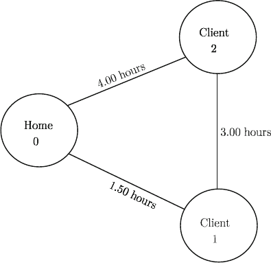
clients buying the item or not. Now, consider the following example. There are two

clients with probability of buying 0.3and0.8 , respectively and traveling times

(including service) as in the graph of Figure 1.

Assume the day starts at 8

A.M. If the sequence is (1,2) , the ﬁrst stage goes

from 8 to 9:30. The second stage starts at 9:30 and ﬁnishes either at 11

A.M. if 1

buys or 4:30

P. M . otherwise. If the sequence is (2,1) , the ﬁrst stage goes from 8

to 12:00, the second stage starts at 12:00 and ﬁnishes either at 4:00

P. M . or at 4:30

P. M . Thus, the ﬁrst stage if sequence (2,1) is chosen may sometimes end after the

second stage is ﬁnished when (1,2) is chosen if Client 1 buys the item.

2.4 Two-Stage Program with Fixed Recourse 59

Fig. 1 Traveling salesperson example.

2.4 Two-Stage Program with Fixed Recourse

The classical two-stage stochastic linear program with ﬁxed recourse (originated by

Dantzig [1955] and Beale [1955]) is the problem of ﬁnding

minz = c

x + E

[minq(

)

)] (4.1)

s. t. Ax = b , (4.2)

)x +Wy(

)=h(

) , (4.3)

x ≥0 ,y(

) ≥0 . (4.4)

As in the previous section, a distinction is made between the ﬁrst stage and the

second stage. The ﬁrst-stage decisions are represented by the n

×1 vector x .

Corresponding to x are the ﬁrst-stage vectors and matrices c , b ,and A , of sizes

×1, m

×1,and m

×n

, respectively. In the second stage, a number of random

events

∈

may realize. For a given realization

, the second-stage problem

data q(

) , h(

) and T(

) become known, where q(

) is n

×1, h(

) is

×1,and T(

) is m

×n

Each component of q , T ,and h is thus a possible random variable. Let T

i·

(

)

be the i th row of T (

) . Piecing together the stochastic components of the second-

stage data, we obtain a vector

(

)=(q(

)

,h(

)

1·

(

),...,T

(

)) , with

potentially up to N = n

+(m

×n

) components. As indicated before, a single

random event

(or state of the world) inﬂuences several random variables, here,

all components of

60 2 Uncertainty and Modeling Issues

Let also

⊂ ℜ

be the support of ξ , that is, the smallest closed subset in

ℜ

such that P(

)=1 . As just said, when the random event

is realized, the

second-stage problem data, q , h ,and T , become known. Then, the second-stage

decision y(

) or (y(

,x)) must be taken. The dependence of y on

is of a

completely different nature from the dependence of q or other parameters on

.It

is not functional but simply indicates that the decisions y are typically not the same

under different realizations of

. They are chosen so that the constraints (4.3)and

(4.4) hold almost surely (denoted a.s.), i.e., for all

∈

except perhaps for sets

with zero probability. We assume random constraints to hold in this way throughout

this book unless a speciﬁc probability is given for satisfying constraints.

The objective function of (4.1) contains a deterministic term c

x and the expec-

tation of the second-stage objective q(

)

) taken over all realizations of the

random event

. This second-stage term is the more difﬁcult one because, for each

,thevalue y(

) is the solution of a linear program. To stress this fact, one some-

times uses the notion of a deterministic equivalent program. For a given realization

,let

Q(x,

(

)) = min

{q(

)

y |Wy = h(

) −T(

)x,y ≥0} (4.5)

be the second-stage value function. Then, deﬁne the expected second-stage value

function

Q(x)=E

Q(x,

(

)) (4.6)

and the deterministic equivalent program (DEP)

minz = c

x + Q(x) (4.7)

s. t. Ax = b ,

x ≥0 .

(4.8)

This representation of a stochastic program clearly illustrates that the major differ-

ence from a deterministic formulation is in the second-stage value function. If that

function is given, then a stochastic program is just an ordinary nonlinear program.

Formulation (4.1)–(4.4) is the simplest form of a stochastic two-stage program.

Extensions are easily modeled. For example, if ﬁrst-stage or second-stage decisions

are to be integers, constraint (4.4) can be replaced by a more general form:

x ∈ X , y(w) ∈Y ,

where X = Z

and Y = Z

. Similarly, nonlinear ﬁrst-stage and second-stage ob-

jectives or constraints can easily be incorporated.

2.4 Two-Stage Program with Fixed Recourse 61

Examples of recourse formulation and interpretations

The deﬁnition of ﬁrst stage versus second stage is not only problem dependent but

also context dependent. We illustrate different examples of recourse formulations

for one class of problems: the location problem.

Let i = 1,...,m index clients having demand d

for a given commodity. The

ﬁrm can open a facility (such as a plant or a warehouse) in potential sites j =

1,...,n . Each client can be supplied from an open facility where the commodity is

made available (i.e., produced or stored). The problem of the ﬁrm is to choose the

number of facilities to open, their locations, and market areas to maximize proﬁt or

minimize costs.

Let us ﬁrst present the deterministic version of the so-called simple plant location

or uncapacitated facility location problem. Let x

be a binary variable equal to one

if facility j is open and zero otherwise. Let c

be the ﬁxed cost for opening and

operating facility j and let v

be the variable operating cost of facility j .Let y

be the fraction of the demand of client i served from facility j and t

be the unit

transportation cost from j to i .

All costs and proﬁts should be taken in conformable units, typically on a yearly

equivalent basis. Let r

denote the unit price charged to client i and q

=(r

−

−t

be the total revenue obtained when all of client i ’s demand is satisﬁed

from facility j . Then the simple plant location problem or uncapacitated facility

location problem (UFLP) reads as follows:

UFLP: max

x,y

z(x,y)=−

∑

j= 1

∑

i=1

∑

j= 1

(4.9)

s. t.

∑

j= 1

≤ 1 , i = 1,...,m , (4.10)

0 ≤ y

≤ x

, i = 1,...,m , j = 1,...,n , (4.11)

∈{0,1} , j = 1,...,n . (4.12)

Constraints (4.10) ensure that the sum of fractions of clients i ’s demand served

cannot exceed one. Constraints (4.11) ensure that clients are served only through

open plants.

It is customary to present the uncapacitated facility location in a different canon-

ical form that minimizes the sum of the ﬁxed costs of opening facilities and of the

transportation costs plus possibly the variable operating costs. (There are several

ways to arrive at this canonical representation. One is to assume that unit prices are

much larger than unit costs in such a way that demand is always fully satisﬁed.) This

presentation more clearly stresses the link between the deterministic and stochastic

cases.

In the UFLP, a trade-off is sought between opening more plants, which results

in higher ﬁxed costs and lower transportation costs and opening fewer plants with

the opposite effect. Whenever the optimal solution is known, the size of an open

62 2 Uncertainty and Modeling Issues

facility is computed as the sum of demands it serves. (In the deterministic case, it is

always optimal to have each y

equal to either zero or one.) The market areas of

each facility are then well-deﬁned.

The notation x

for the location variables and y

for the distribution variables

is common in location theory and is thus not meant here as ﬁrst stage and second

stage, respectively, although in some of the models it is indeed the case.

Several parameters of the problem may be uncertain and may thus have to be

represented by random variables. Production and distribution costs may vary over

time. Future demands for the product may be uncertain.

As indicated in the introduction of the section, we will now discuss various sit-

uations of recourse. It is customary to consider that the location decisions x

are

ﬁrst-stage decisions because it takes some time to implement decisions such as mov-

ing or building a plant or warehouse. The main modeling issue is on the distribution

decisions. The ﬁrm may have full control on the distribution, for example, when the

clients are shops owned by the ﬁrm. It may then choose the distribution pattern after

conducting some random experiments. In other cases, the ﬁrm may have contracts

that ﬁx which plants serve which clients, or the ﬁrm may wish ﬁxed distribution pat-

terns in view of improved efﬁciency because drivers would have better knowledge

of the regions traveled.

a. Fixed distribution pattern, ﬁxed demand, r

stochastic

Assume the only uncertainties are in production and distribution costs and prices

charged to the client. Assume also that the distribution pattern is ﬁxed in advance,

i.e., is considered ﬁrst stage. The second stage then just serves as a measure of

the cost of distribution. We now show that the problem is in fact a deterministic

problem in which the total revenue q

=(r

−v

−t

can be replaced by its

expectation. To do this, we formally introduce extra second-stage variables w

with the constraint w

(

)=y

for all

. We obtain

max −

∑

j= 1

+ E

∑

i=1

∑

j= 1

(

)

s.t. (4.10), (4.11), (4.12), and

(

)=y

, i = 1,...,m , j = 1,...,n ∀

. (4.13)

By (4.13), the second-stage objective function can be replaced by

∑

i=1

∑

j= 1

(

2.4 Two-Stage Program with Fixed Recourse 63

∑

i=1

∑

j= 1

(

because y

is ﬁxed and summations and expectation can be interchanged. The

problem is thus the deterministic problem

max −

∑

j= 1

∑

i=1

∑

j= 1

(

))y

s.t. (4.10), (4.11), (4.12).

Although there exists uncertainty about the distribution costs and revenues, the

only possible action is to plan in view of the expected costs.

b. Fixed distribution pattern, uncertain demand

Assume now that demand is uncertain, but, for some of the reasons cited earlier,

the distribution pattern is ﬁxed in the ﬁrst stage. Depending on the context, the

distribution costs and revenues (v

) may or may not be uncertain.

We deﬁne y

= quantity transported from j to i , a quantity no longer deﬁned

as a function of the demand d

, because demand is now stochastic. For simplicity,

we assume that a penalty q

is paid per unit of demand d

which cannot be satisﬁed

from all quantities transported to i (they might have to be obtained from other

sources) and a penalty q

−

is paid per unit on the products delivered to i in excess

of d

(the cost of inventory, for example). We thus introduce second-stage variables:

−

(

)= amount of extra products delivered to i in state

; w

(

)= amount

of unsatisﬁed demand to i in state

The formulation becomes

max−

∑

j= 1

∑

i=1

∑

j= 1

(−v

−t

))y

+ E

[−

∑

i=1

(

)

−

∑

i=1

−

(

)] + E

∑

i=1

(

) (4.14)

s. t.

∑

i=1

≤ Mx

, j = 1,...,n , (4.15)

(

) −w

−

(

)=d

(

) −

∑

j= 1

, i = 1,...,m , (4.16)

∈{0,1} , 0 ≤y

, w

(

) ≥ 0 ,w

−

(

) ≥0 ,

i = 1,...,m , j = 1,...,n . (4.17)

This model is a location extension of the transportation model of Williams [1963].

The objective function contains the investment costs for opening plants, the expected