Birge J.R., Louveaux F. Introduction to Stochastic Programming

Подождите немного. Документ загружается.

144 3 Basic Properties and Theory

u(x + n)=u(x) −

n−1

∑

k=0

(1 −F(x + k)) (3.16)

and

v(x + n)=v(x)+

∑

k=1

F(x+ k)) . (3.17)

Corollary 27. Let ξ be a discrete random variable with support

∈ Z.Then

u(x)=



−x−

∑

−1

k=x

F(k) if x < 0 ,

−x+

∑

x−1

k=0

F(k) if x ≥0 .

Proof: Because

∈ Z , F(t)=F(t) ,forall t ∈ ℜ . Hence, u(x)=u(x) for

all x ∈R .Now, u(0)=

. Then apply (3.16) to obtain the result.

Corollary 28. Let ξ be a discrete random variable with support

∈ Z.Then

v(x)=



−

∑

−1

k=x

F(k) if x < 0 ,

−

∑

x−1

k=0

F(k) if x ≥ 0 .

Thus, here the ﬁnite computation comes from the ﬁniteness of x .

Case d. Finally, we may have a random variable that does not fall in any of the

given categories. We may then resort to approximations.

Theorem 29. Let ξ be a random variable with cumulative distribution function,

F.Then

ˆu(x) ≤ u(x) ≤ ˆu(x)+1 −F(x) . (3.18)

Proof: The ﬁrst inequality was given in (3.13). Because 1−F(t) is nonincreasing,

we have for any x ∈ ℜ and any k ∈{1, 2,...} that

1 −F(x + k) ≤ 1 −F(t) , t ∈ [x + k −1, x + k) .

Hence,

∞

∑

k=1

(1 −F(x + k)) ≤



∞

(1 −F(t)) dt .

Adding 1 −F(x) to both sides gives the desired result.

Theorem 30. Let ξ be a random variable with cumulative distribution function

F . Let n be some integer, n ≥1 . Deﬁne

3.3 Stochastic Integer Programs 145

(x)=

n−1

∑

k=0

(1 −F(x + k)) + ˆu(x + n) . (3.19)

Then

(x) ≤ u(x) ≤ u

(x)+1 −F(x + n) . (3.20)

Proof: The proof follows directly from Theorem 29 and Formula (3.16).

To approximate u(x) within an accuracy

, we have to compute the ﬁrst n

terms in u(x) ,where n is chosen so that F(x + n) ≥ 1 −

and ˆu(x + n) ,which

involves computing one integral.

Example 10

Let ξ follow a normal distribution with mean

and variance

, i.e., N(

) ,

with cumulative distribution function F and probability density function f .Inte-

grating by parts, one obtains:

(x)=

n−1

∑

k=0

(1 −F(x + k)) +



∞

x+n

(1 −F(t)) dt

n−1

∑

k=0

(1 −F(x + k)) −(x + n)(1 −F(x + n)) +



∞

x+n

tf(t) dt .

Using tf(t)=

f (t) −



(t) , it follows that

(x)=

n−1

∑

k=0

(1 −F(x + k)) + (

−x−n)(1 −F(x + n)) +

f (x + n) .

Similar results apply for v(x) .

Theorem 31. Let

be a random variable with cumulative distribution function

F(t)=P {

< t}.Then

ˆv(x) ≤ v(x) ≤ ˆv(x)+

F(x) . (3.21)

Let n be some integer, n ≥1 . Deﬁne

(x)=

n−1

∑

k=0

F(x−k)+ ˆv(x −n) . (3.22)

Then

(x) ≤ v(x) ≤ v

(x)+

F(x −n) . (3.23)

146 3 Basic Properties and Theory

Example 10 (continued)

Let ξ follow an N(

) distribution, with cumulative distribution function F

and probability density function f .Then

(x)=

n−1

∑

k=0

F(x−k)+(x −n −

)F(x −n)+

f (x −n) .

As a conclusion, expected shortage, expected surplus, and thus simple integer re-

course functions can be computed in ﬁnitely many steps either in an exact manner or

within a prespeciﬁed tolerance

. Deeper studies of continuity and differentiability

properties of the recourse function can be found in Stougie [1987], Louveaux and

van der Vlerk [1993], and Schultz [1993].

c. Probabilistic constraints

Probabilistic constraints involving integer decision variables may generally be treated

in exactly the same manner as if they involved continuous decision variables. One

need only take the intersection of their deterministic equivalents with the integrality

requirements. The question is then how to obtain a polyhedral representation of this

intersection. This problem sometimes has quite nice solutions.

Example 11: Covering

Consider an example where one can invest in any one of n projects in order to

obtain at least b units of a good. Projects could be mines needed to extract at least

b tons of ore per year, or buildings to let in order to obtain at least b thousands of

rent per year

Let x

be the binary variable representing the decision to invest ( x

= 1 ) or not

( x

= 0 ) in project i . In a deterministic setting, the yield of a project is the quantity

and the requirement of b units is described by the deterministic constraint

∑

i=1

≥ b . (3.24)

Now, assume the yields are in fact random. This may come from operational difﬁ-

culties in a mine or on some ﬂoors of the buildings remaining vacant for a period of

time. Then, a typical probabilistic constraint would be



∑

i=1

≥ b



≥

, (3.25)

3.3 Stochastic Integer Programs 147

where ξ

is the random yield of project i .

Due to the binary nature of the decision variables x

, this constraint is equivalent



∑

i∈S

≥ b



≥

(3.26)

where S is some subset of {1,...,n} representing the selected projects.

Now, if the random variables ξ

follow a Poisson distribution with parameter a

then ξ

∑

i∈S

follow a Poisson distribution with parameter

∑

i∈S

and (3.26)

is equivalent to

P (ξ

≥ b) ≥

. (3.27)

As b and

are given and ξ

is known to follow a Poisson distribution, this cor-

responds to ﬁnding in the table of the cumulative Poisson distribution the smallest

parameter value for which (3.27) holds. Let B be this value. Then (3.27) is equiva-

lent to

∑

i∈S

≥ B

∑

i=1

≥ B . (3.28)

Thus, the probabilistic constraint (3.25) has the linear equivalent (3.28). This

linear equivalent has exactly the same form as (3.24) with b replaced by a larger

quantity B .

Example 12

Assume one has ﬁve projects with expected yields 2 , 2.5, 4, 4.5, and 7. The

level b = 9 is requested. The deterministic constraint based on expected yields is

2 x

+ 2.5 x

+ 4 x

+ 4.5 x

+ 7 x

≥ 9 .

The constraint can be satisﬁed with Project 5 and any other, or by Projects 1, 2 and

4, for instance.

If yields are random and follow a Poisson distribution and if the level of 9 must

be obtained with probability 90%, then a value of B = 13 is found in the Poisson

table and (3.28) gives the linear equivalent:

2 x

+ 2.5 x

+ 4 x

+ 4.5 x

+ 7 x

≥ 13 .

148 3 Basic Properties and Theory

Example 13: Routing

Let V = {v

,...,v

} be a set of vertices, typically representing customers. Let

represent the depot and let V

= V ∪{v

}. A route is an ordered sequence L =

= 0,i

,...,i

k+1

= 0}, with k ≤ n , starting and ending at the depot and

visiting each customer at most once. Clearly, if k < n , more than one vehicle is

needed to visit all customers. Assume a vehicle of given capacity C follows each

route, collecting customers’ demands d

. If demands d

are random, it may turn

out that at some point of a given route, the vehicle cannot load a customer’s demand.

This is clearly an undesirable feature, which is usually referred to as a failure of the

route. A probabilistic constraint for the capacitated routing requires that only routes

with a small probability of failure are considered feasible:

P(failure on any route) ≤

, (3.29)

where we note that here and elsewhere we use

as an upper bound on a probability

(instead of a lower bound as in (2.1)) in following typical usage in the context.

We now show, as in Laporte, Louveaux, and Mercure [1989], that any route that

violates (3.29) can be eliminated by a linear inequality. For any route L ,let S =

,...,i

} be the index set of visited customers. Violation of (3.29) occurs if

P (

∑

i∈S

> C) >

. (3.30)

Let V

(S) denote the smallest number of vehicles required to serve S so that the

probability of failure in S does not exceed

, i.e., V

(S) is the smallest integer

such that

P (

∑

i∈S

> C ·V

(S)) ≤

. (3.31)

Now, let

S denote the complement of S versus V

,i.e.,

S = V

\S . Then the follow-

ing subtour elimination constraint imposes, in a linear fashion, that at least V

(S)

vehicles are needed to cover demand in S :

∑

i∈S, j∈

S or i∈

S, j∈S

≥ 2V

(S) , (3.32)

where, as usual, x

= 1whenarcij is traveled in the solution and x

= 0other-

wise. It follows that routes that violate (3.29) can be eliminated when needed by the

linear constraint (3.32). Observe that this result is obtained without any assumption

on the random variables. Also observe that (3.32) is not the deterministic equivalent

of (3.29). This should be clear from the fact that an analytical expression for (3.29)

is difﬁcult to write. Finally, observe that in practice, as for many random variables,

the probability distribution of

∑

i∈S

is easily obtained. The computation of V

(S)

in (3.31) poses no difﬁculty. Additional results appear in the survey on stochastic

vehicle routing by Gendreau, Laporte, and S´eguin [1996].

3.4 Multistage Stochastic Programs with Recourse 149

Exercises

1. Consider the following second-stage integer program:

Q(x,

)=max{4y

+ y

| y

+ y

≤

x,0 ≤y

≤ 2,0 ≤y

≤ 1,y integer} .

(a) Obtain y

∗

, y

∗

,and Q(x,

) as Gomory functions.

(b) Consider

= 1.Observethat Q(x,1) is piecewise constant on four pieces

( x < 1, 1≤ x < 2, 2≤ x < 3, 3≤ x ).

pieces ( x < 0.5, 0.5 ≤x < 1, 1≤ x < 1.5, 1.5 ≤ x ). Check the noncon-

cavity of Q(x) . Observe that Q (x) is concave on each piece separately,

but that Q(x) is not (compare, e.g., Q(1) to 1/2Q(3/4)+1/2Q(5/4) ).

2. Consider ξ uniformly distributed over [0, 1] and 0 ≤x ≤1.Showthat u(x)+

v(x)=1.

3. Consider ξ uniformly distributed over [0, 2] .

(a) Compute u(x) directly from Deﬁnition (3.9) and check with the result in

Example 8. Observe that u(x) is piecewise linear, convex, and continuous.

(b) Compute ˆu(x) .

4. Consider ξ that is Poisson distributed with parameter three. Compute u(3) .

5. (a) Let ξ be normally distributed with mean zero and variance one. What is

the accuracy level of u

(0) versus u(0) ?

(b) Let ξ be normally distributed with mean

and variance

. Show that

) is independent of

. Is the accuracy of u

(

) , n given, increasing

or decreasing with

6. Consider Example 11. In this example, a probabilistic constraint has a determin-

istic linear equivalent.

(a) Does this also hold if x

are integer variables, instead of binary variables?

(b) Does this also hold if the random variables ξ

are normally distributed with

mean a

and variance

3.4 Multistage Stochastic Programs with Recourse

The previous sections in this chapter concerned stochastic programs with two stages.

Most practical decision problems, however, involve a sequence of decisions that re-

act to outcomes that evolve over time. In this section, we will consider the stochastic

programming approach to these multistage problems. We present the same basic re-

sults as in previous sections. We describe the basic structure of feasible solutions,

150 3 Basic Properties and Theory

objective values, and conditions for optimality. We begin again with the linear, ﬁxed

recourse, ﬁnite horizon framework because this model has been the most widely

implemented. We then continue with more general approaches.

We start with implicit nonanticipativity constraints as in the previous sections.

The multistage stochastic linear program with ﬁxed recourse then takes the follow-

ing form (where we note that transposes are suppressed when they are clear from

context to avoid excessive notation):

minz = c

+ E

[minc

(

)+···+ E

[minc

(

)]...]

s. t. W

= h

(

)=h

(

) ,

···

H−1

(

H−1

(

H−1

)+W

(

)=h

(

) ,

≥ 0; x

(

) ≥ 0 , t = 2,...,H ;

(4.1)

where c

is a known vector in ℜ

, h

is a known vector in ℜ

(

)

(

)

(

)

t−1

1·

(

),...,T

t−1

) is a random N

-vector deﬁned on (

,P)

(where

⊂

t+1

)forall t = 2,...,H , and each W

is a known m

×n

matrix.

The decisions x depend on the history up to time t , which we indicate by

.We

also suppose that

is the support of ξ

For the ﬁnancial planning problem in Section 1.2, these parameters are:

(

)=0,t = 1,...,H −1;

(

)=(q,−r);

= e

,t = 1,...,H −1;

=[1 −1],t = 1,...,H −1;

= −

(

)

,t = 1,...,H;

= b;

= 0,t = 1,...,H −1;

= −G.

We ﬁrst describe the deterministic equivalent form of this problem in terms of a

dynamic program. If the stages are 1 to H , we can deﬁne states as x

(

) . Noting

that the only interaction between periods is through this realization, we can deﬁne a

dynamic programming type of recursion. For terminal conditions, we have:

H−1

(

)) = minc

(

)

s. t. W

(

)=h

(

) −T

H−1

(

H−1

(

) ≥ 0 .

(4.2)

3.4 Multistage Stochastic Programs with Recourse 151

For the ﬁnancial planning problem in Section1.2,given x

H−1

and

(

) ,(4.2)

has an optimal solution given by

(

)=(y(

),w(

)) = ((G −

(

)

H−1

(

))

(

)

H−1

(

) −G)

Solutions for other stages can be obtained with a backward recursion, let-

ting Q

t+1

)=E

t+1

(

))] for all t to obtain the recursion for

t = 2,...,H −1,

t−1

(

)) = minc

(

)+Q

t+1

)

s. t. W

(

)=h

(

) −T

t−1

(

t−1

(

) ≥ 0 ,

(4.3)

where x

indicates the state of the system. Other state information in terms of the

realizations of the random parameters up to time t should be included if the dis-

tribution of ξ

is not independent of the past outcomes. In the ﬁnancial planning

case, the value function, Q

t+1

) , represents the expected utility of choosing the

asset allocations given by x

in the t th period and choosing optimal allocations in

all subsequent periods.

The value we seek is:

minz = c

+ Q(x

)

s. t. W

= h

≥ 0 ,

(4.4)

which has the same form as the two-stage deterministic equivalent program. The

examples of this formulation in Chapter 1 for ﬁnancial planning and capacity expan-

sion could then be re-cast as two-stage problems if the second-stage value function

Q(x

) can be found.

We would again like to obtain properties of the problems in (4.2)–(4.4) that allow

uses of mathematical programming procedures such as decomposition. We concen-

trate ﬁrst on the form of the feasible regions for problems (4.3). Let these be

= {x

| Q

t+1

) < ∞} .

We have the following result which helps in the development of several algorithms

for multistage stochastic programs.

Theorem 32. The sets K

and functions Q

t+1

) are convex for t = 1,...,H −1

and, if

is ﬁnite for t = 1,...,H,then K

and Q

t+1

) are polyhedral.

Proof: Proceed by induction. Because Q

H−1

(

)) is convex for all

(

) ,

so too is Q

H−1

) . We can then carry this back to each t < T −1.Thesameap-

plies for the polyhedrality property because ﬁnite numbers of realizations lead to

each Q

t+1

) ’s being the sum of a ﬁnite number of polyhedral functions, which is

then polyhedral.

152 3 Basic Properties and Theory

We note that we may also describe the feasibility sets K

in terms of intersections

of feasibility sets for each outcome if we have ﬁnite second moments for ξ

in each

period. This result is also true when we have a ﬁnite number of possible realizations

of the future outcomes. In this case, the set of possible future sequences of outcomes

are called scenarios.

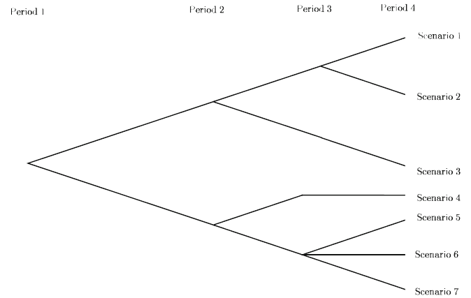
The description of scenarios is often made on a tree such as that in Figure 4.

Here, there are seven scenarios that are evident in the last stage ( H = 4 ). In previous

stages ( t < 4 ), we have a more limited number of possible realizations, which we

call the stage t scenarios. Each of these period t scenarios is said to have a single

ancestor scenario in stage ( t −1 ) and perhaps several descendant scenarios in stage

( t + 1 ). We note that different scenarios at stage t may correspond to the same ξ

realizations and are only distinguished by differences in their ancestors.

Fig. 4 A tree of seven scenarios over four periods.

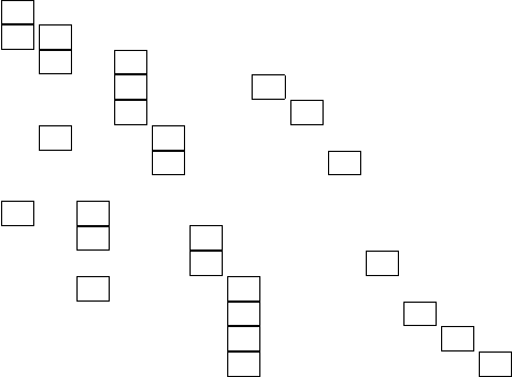
The deterministic equivalent program to (4.1) with a ﬁnite number of scenar-

ios is still a linear program. It has the structural form indicated in Figure5,where

subscripts indicate different scenario realizations for the T

matrices. This is often

called arborescent form and can be exploited in large-scale optimization approaches

as in Kallio and Porteus [1977]. A difﬁculty is still, however, that these problems

become extremely large as the number of stages increases, even if only a few real-

izations are allowed in each stage.

In some problems, however, we can avoid much of this difﬁculty if the interac-

tions between consecutive stages are sufﬁciently weak. This is the case in the ca-

pacity expansion problem described in Section 1.3. Here, capacity carried over from

3.4 Multistage Stochastic Programs with Recourse 153

Fig. 5 The deterministic equivalent matrix for a problem with seven scenarios in four periods.

one stage to the next is not affected by the demand in that stage. Decisions about

the amount of capacity to install can be made at the beginning and then the future

only involves reactions to these outcomes. Problems with this form are called block

separable as mentioned in Section 1.3. Formally, we have the following deﬁnition

for block separability (see Louveaux [1986]).

Deﬁnition 33. A multistage stochastic linear program (4.1) has block separable

recourse if for all periods t = 1,...,H and all

, the decision vectors, x

(

) ,

can be written as x

(

)=(w

(

),y

(

)) where w

represents aggregate level

decisions and y

represents detailed level decisions. The constraints also follow

these partitions:

1. The stage t objective contribution is c

(

)=r

(

)+q

(

) .

2. The constraint matrix W

is block diagonal:



0 T



. (4.5)

3. The other components of the constraints are random but we assume that for

each realization of

(

) and h

(

) can be written:

(



(

) 0

(

) 0



and h

(



(

)

(

)



, (4.6)

where the zero components of T

correspond to the detailed level variables.

To put the capacity expansion problem in Section 1.3 into this framework, we

keep information about the the installed capacity from the current and previous