Birge J.R., Louveaux F. Introduction to Stochastic Programming

Подождите немного. Документ загружается.

314 7 Stochastic Integer Programs

b. Disjunctive cuts

One way to overcome these difﬁculties is through the use of disjunctive cuts, as

we now explain. Section 7.8c. provides a short reminder of disjunctive cuts, with a

proof and some examples.

Proposition 11. If P

= {x ∈ ℜ

x ≥b

} for i = 0,1 are two nonempty polyhe-

dra, then

x ≥

is a valid inequality for co(P

∪P

) if and only if there exists

≥ 0 such that

≥ (u

)

and

≤ (u

)

for i = 0,1 .

This proposition provides a way of convexifying the union of two sets. It will be

used in this form at the end of this section. It is also used to realize the disjunction

for a fractional variable.

Let P = {y ∈ ℜ

|Wy ≥ d , y ≤ e} be a particular second stage LP-relaxation

(i.e. for one particular

and one particular h −Tx

= d ). Assume that, at the

solution of the second-stage LP-relaxation, some second-stage binary variable y

takes a fractional value. Instead of a classical branching y

≤0versusy

≥1 , one

can consider the disjunction P

= P ∩{y ∈ ℜ

| y

≤ 0} and P

= P ∩{y ∈ ℜ

≥ 1} . Specializing Proposition 11 (with speciﬁc dual variables for each type of

constraint and with each constraint under the ≥ format), one obtains the following.

Proposition 12. The inequality

y ≥

is valid if and only if there exists

≥ 0 for i = 0,1 such that

≥ (u

)

W −v

−w

≥ (u

)

W −v

+ w

≤ (u

)

d −e

≤ (u

)

d −e

+ w

A disjunctive cut is obtained by solving an LP consisting of maximizing the

violation

−

, under the constraints deﬁned in Proposition 12, where y

the current solution of the second stage LP. To be bounded, this LP needs some

normalizing. One possibility is to take −1 ≤

≤ 1, −e ≤

≤ e .

Proposition 12 is used in deterministic integer programs to generate one disjunc-

tive cut. It is desired now to ﬁnd one such cut for each realization

. The idea of

the so-called common cut coefﬁcient technique consists of obtaining an inequality

y ≥

where the coefﬁcients

for the variables remain the same independently

of k and only the r.h.s.’s are dependent on k .

Proposition 13 (Common Cut Coefﬁcient or C

). The inequality

y ≥

valid for k = 1,...,K if and only if there exists u

≥ 0 for i = 0,1 such that

≥ (u

)

W −v

−w

≥ (u

)

W −v

+ w

7.4 Reformulation 315

≤ (u

)

−e

≤ (u

)

−e

+ w

where d

= h

−T

In practice, the cut is obtained by solving an LP consisting of maximizing the

expected violation

∑

k=1

(

−

) under the constraints deﬁned in Proposi-

tion 13, where y

is the second-stage solution associated to d

. As above, we may

use the normalization −1 ≤

≤ 1, −e ≤

≤ e . This LP is called the C

−LP

or C

−LP(W, d

) if one needs to specify the problem data.

Example 5 (continued)

Consider again the second-stage program:

Q(x,

)=min 3y

+ 7y

+ 9y

+ 6y

s. t. 2y

+ 4y

+ 5y

+ 3y

≥ h −Tx ,

,...,y

∈{0,1} ,

with the two realizations h−T.x = 10−2x

−4x

and 11−4x

−3x

for k = 1,2,

with probability 0.25 and 0.75 , respectively.

Consider the current iterate x

=(0.3,0.6)

. The corresponding second-stage

r.h.s. values d

= h

−T

are 7 and 8 , respectively for k = 1, 2 . The solutions

of the second-stage LP relaxations are y =(1, 1,0.2,0)

and y =(1,1,0.4,0)

for

the two realizations. The disjunction is made on y

as it is fractional in both cases.

Taking the objective of maximizing the expected violation

∑

k=1

(

−

) and

the normalization as above, the (C

-LP) problem reads as follows:

-LP) z =max 0.25

+ 0.75

−

−0.35

s. t.

≥ 2u

−v

≥ 2u

−v

≥ 4u

−v

≥ 4u

−v

≥ 5u

−v

−w

≥ 5u

−v

+ w

≥ 3u

−v

≥ 3u

−v

≤ 7u

−v

≤ 7u

−v

+ w

≤ 8u

−v

≤ 8u

−v

+ w

−e ≤

≤ e , −1 ≤

≤1 , u,v,w ≥ 0 .

316 7 Stochastic Integer Programs

Its optimal solution is z = 0.35 , u

= 1/3, v

=(2/3, 4/3, 0,0)

, u

= 0, v

(0,0, 0,0)

, w

= 1, w

= 2/3,

=(0,0, 2/3,1)

= 1/3,

= 2/3.The

two cuts are 2/3y

+ y

≥ 1/3, 2/3y

+ y

≥ 2/3,for k = 1,2 , respectively.

At the current second-stage solutions, the two cuts are violated by an amount

of 0.6/3and1.2/3 , respectively. The expected violation corresponds to the value

0.35 of the objective of C

−LP .Giventhe u , v , w values, one can check that

≤ min{1/3,2/3} and

≤ min{2/3,2/3}.

We now look of how to make these values dependent on the ﬁrst-stage decision

variables.

c. First-stage dependence

Consider the C

cut for a given k . We have seen that

y ≥

is valid for

≤ (u

)

−e

≤ (u

)

−e

+ w

where d

= h

−T

If instead of considering a ﬁxed d

,welet x vary, we obtain a cut

y ≥

(x)

whose r.h.s depends on x . This cut remains valid for

(x) ≤ (u

)

−T

x) −e

(x) ≤ (u

)

−T

x) −e

+ w

With

, u , v and w unchanged, it sufﬁces indeed to take a sufﬁciently small value

(x) to obtain a valid cut.

To simplify notations, let

=(u

)

−e

=(u

)

−e

+ w

and

=(u

)

for i = 0,1 . Thus,

y ≥ min{

−

where the index k is omitted in the r.h.s. even if the data are dependent on k .

Due to the min operation, the cut is nonlinear and needs convexiﬁcation. This

can be achieved through a disjunction with the two sets

= {x ∈ ℜ

≥ 0 | Ax ≥b ,

≥

−

x} ,

= {x ∈ ℜ

≥ 0 | Ax ≥b ,

≥

−

x} ,

where

is an extra variable representing the minimum of the two expressions.

The RHS(k) problem consists of ﬁnding r

≥ 0fori = 0,1and(

) s.t.

≥ (r

)

A +

7.4 Reformulation 317

≥ (r

)

A +

≤ (r

)

b +

≤ (r

)

b +

, s

≤ 1 .

These inequalities are written down assuming a value of 1 for the coefﬁcient of

,toformacut

≥

−

x . This is an appropriate form of normalization. The

solution is obtained from an LP with the objective of maximizing max

−

The ﬁnal cut is

y ≥

−

x .

The notation RHS(k) is a reminder that the r.h.s. of the resulting cut is valid for

one given k . When needed, the notation

y ≥

−

x is then used to represent

the cut obtained for one speciﬁc k .

Example 5 (continued)

Assume a single ﬁrst stage constraint 4x

+ 6x

≤ 5 and, as above, a current it-

erate x

=(0.3,0.6)

. The solution of the C

−LP includes u

= 1/3, v

(2/3,4/3,0,0)

, u

= 0, v

=(0,0, 0,0)

, w

= 1, w

= 2/3.

Consider k = 1 . Thus, h −Tx = 10 −2x

−4x

. We obtain

= 1/3p10 −

6/3 = 4/3and

=(2/ 3,4/3)

for i = 0and

= 2/3and

=(0, 0)

for

i = 1. RHS(1) consists in convexifying min{4/3 −2/3x

−4/3x

,2/3} under

+ 6x

≤ 5, x

≥ 0 . Using the objective max

−

and the proposed

normalization of the coefﬁcient of

, we obtain:

RHS(1) z = max

−0.3

−0.6

s. t.

≥−4r

+ 2/3s

≥−4r

≥−6r

+ 4/3s

≥−6r

≤−5r

+ 4/3s

≤−5r

+ 2/3s

0 ≤r

, 0 ≤s

≤ 1 .

The optimal solution is z = 0.92/3,

= 2/3,

= 0.4/3,

= 1.6/3. The

disjunctive cut for k = 1 is thus 2/3y

+ y

≥ 2/3 −0.4/3x

−1.6/3x

d. An algorithm

For simplicity, we present an algorithm with second-stage reformulation for the

case when the ﬁrst-stage variables are continuous and assuming relatively com-

plete recourse. Such an algorithm is a direct extension of the L -shaped method

of Chapter 5, with an extended Step 3 for the construction of the Benders cuts.

318 7 Stochastic Integer Programs

L -Shaped Algorithm with Second-stage Reformulation

Step 0.Set s =

= 0.Set W

= W , h

= h , T

= T .

Step 1 and Step 2: unchanged.

Step 3.

(a) Solve the LP-relaxation C(x,

)=min

y |W

y ≥ h

−T

, 0 ≤y ≤e}

for k = 1,...,K .

(b) Select some component j s.t. y

is fractional for at least one k . (If none ex-

ists, let W

= W

, h

= h

, T

= T

and go to (f) with unchanged

multipliers).

−LP(W

) with d

= h

−T

. Append the solution

to the

matrix W

to form W

(d) Solve RHS(k) for k = 1,...,K . For each k , append

to h

to form h

+1,k

and append

to the matrix T

to form T

+1,k

(e) Solve the LP-relaxation C(x,

)=min

y |W

y ≥h

+1,k

−T

+1,k

, 0 ≤

y ≤e} for k = 1,...,K .

(f) Use the dual multipliers to generate an L -Shaped cut as in (5.1.6)and(5.1.7),

based on h

+1,k

and T

+1,k

(g) Test of optimality or addition of the cut (as in the end of Step 3 in the L -shaped

method).

If one compare the above steps with those of the L -shaped method, the extra

work consists of solving one C

−LP , solving K times a RHS(k) and reoptimiz-

ing the K second-stage relaxations with one extra constraint each. The C

−LP

has 2m

+ 2n

+ 2K + 2 variables and 2n

+ 2K constraints. Each RHS(k) has

+ 2 variables and 2n

+ 2 constraints. The alternative of ﬁnding one possibly

different disjunctive cut for each k not only in the r.h.s. but also in the l.h.s. would

request the solution of K successive LP’s, each having 2m

+ 2n

+ 2 variables

and 2n

+ 2 constraints. The convexiﬁcation of the r.h.s.’s would still require the

solution of KRHS(k) programs having the same dimension as above.

The above algorithm was developed by Sen and Higle [2005]. It can be seen as

an integer L -shaped type of method, with more elaborate steps for the construc-

tion of the cuts. The case of continuous ﬁrst-stage may present some technicalities

that are studied in Ntaimo and Sen [2006a]. The second stage reformulation may

fail to produce natural integer solutions in the second-stage for all k = 1,...,K in

a sufﬁciently fast manner. In such a case, an extra branch-and-bound step in the

second-stage may be needed. A description of this extra feature can be found in Sen

and Sherali [2002]. Reports on computational experiments can be found in Ntaimo

and Sen [2006b].

7.5 Simple Integer Recourse 319

Exercises

1. Take Example 5 and problem RHS(1) . For the current iterate point with y

0.2, y

= 0andx

=(0.3,0.6)

, compare the violation of the disjunctive cut

after convexiﬁcation and the one in the C

−LP solution.

2. Take Example 5. Solve RHS(2) and obtain the cut 2/3y

≥2/3−1.6/3x

3. Take Example 5. Suppose that the ﬁrst-stage constraints are x

≤ 1, x

≤ 1

(instead of the single constraint 4x

+ 6x

≤ 5).Solve RHS(1) and RHS(2)

to obtain the r.h.s. of the disjunctive cuts. What are the violations at the current

iterate point x

=(0.3,0.6)

7.5 Simple Integer Recourse

As seen in Section 3.3, a two-stage stochastic program with simple integer recourse

can be transformed into

min c

x +

∑

i=1

(

)

s. t. Ax = b , Tx=

, x ∈ X ⊂ Z

, (5.1)

where

(

)=q

(

)+q

−

(

) (5.2)

with

(

)=E

−



, (5.3)

deﬁned as the expected shortage, and

(

)=E

−



, (5.4)

deﬁned as the expected surplus. As before, we assume

≥ 0,q

−

≥0 .

Also from Section 3.3, we know that the values of the expected shortage and sur-

plus can be computed in ﬁnitely many steps, either exactly or within a prespeciﬁed

tolerance

Before turning to algorithms, we still need some results concerning the functions

; for simplicity in the exposition we omit the index i . As we also know from

Section 3.3, the function

is generally not convex and is even discontinuous when

ξ has a discrete distribution. It turns out, however, that some form of convexity

exists between function values evaluated in (not necessarily integer) points that are

320 7 Stochastic Integer Programs

integer length apart. Thus, let x

∈ ℜ be an arbitrary point. Let i ∈ Z be some

integer.

Deﬁne x

= x

+ i ,andforany j ∈ Z , j ≤ i , x

= x

+ j . Equivalently, we

may deﬁne

+(1 −

=(i − j)/i .

In the following, we will use x as an argument for

as if Tx= Ix =

without

losing generality. We make T explicit again when we speak of a general problem

and not just the second stage.

Proposition 14. Let x

∈ℜ ,i, j ∈ Z with j ≤ i, x

= x

+ i, x

= x

+ j.Then

) ≤

λΨ

)+(1 −

)

) (5.5)

with

=(i − j)/i.

Proof: We prove that

(x+ 1)−

(x) is a nondecreasing function of x .Weleave

it as an exercise to infer that this is a sufﬁcient condition for (5.5) to hold. Using

(3.3.16)and(3.3.17), we respectively obtain u(x + 1) −u(x)=−(1 −F(x)) and

v(x + 1) −v(x)=

F(x + 1) ,where F is again the cumulative distribution function

of ξ and

F is deﬁned as in Section 3.3. With this,

(x + 1) −

(x)=q

−

F(x+ 1) −q

(1 −F(x)) .

The result follows as q

≥ 0, q

−

≥ 0and

F and F are nondecreasing.

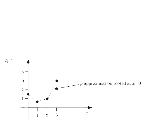
This means that we can draw a piecewise linear convex function through points

that are integer length apart. Such a convex function is called a

-approximation

rooted at x if it is drawn at points x±

integer. In Figures 3 and 4, we provide

the

-approximations rooted at x = 0andx = 0.5 , respectively, for the case in

Example 3.1.

Fig. 3 The

-approximation rooted at x = 0.

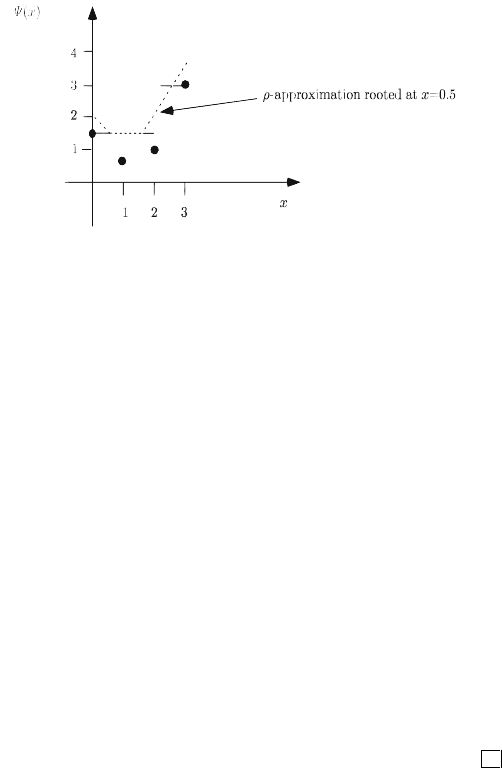
7.5 Simple Integer Recourse 321

Fig. 4 The

-approximation rooted at x = 0.5.

If we now turn to discrete random variables, we are interested in the different pos-

sible fractional values associated with a random variable. As an example, if ξ can

take on the values 0.0, 1.0, 1.2, 1.6, 2.0, 2.2, 2.6,and 3.2 with some given

probability, then the only possible fractional values are 0.0, 0.2, and 0.6. Let

< f

< ···< f

denote the S ordered possible fractional values of ξ .Deﬁne

S+1

= 1 . Let the extended list of fractionals be all points of the form a + f

a ∈ Z ,1≤ s ≤ S . This extended list is a countable list that contains many more

elements than the possible values of ξ . In the example, 0.2, 0.6, 3.0, 3.6, 4.0,

4.2,...areintheextendedlistoffractionalsbutarenotpossiblevaluesof ξ .

Lemma 15. Let ξ be a discrete random variable. Assume that S is ﬁnite. Let

a ∈Z.Then

(x) is constant within the open interval (a + s

,a + s

j+ 1

) ,

(x) ≥ max {

(a + s

j+ 1

)} ,

for all x ∈ (a + s

,a + s

j+ 1

) .

Proof: The proof can be found in Louveaux and van der Vlerk [1993].

The lemma states that

(x) is piecewise constant in the open interval between

two consecutive elements of the extended list of fractionals and that the values in

points between two consecutive elements of that list are always greater than or equal

to the values of

(·) at these two consecutive elements in the extended list. The

reader can easily observe this property in the examples that have already been given.

Corollary 16. Let ξ be a random variable with S = 1 .Let

(·) be a

approximation of

(·) rooted at some point in the support of

.Then

(x) ≤

(x), ∀ x ∈ ℜ.

Moreover,

is the convex hull of the function

322 7 Stochastic Integer Programs

Proof: By Lemma 15,

∀ x ∈ (a,a + 1) ,

(x) ≤ max{

(a),

(a + 1)}= max{

(a),

(a + 1)}≤

(x) .

Thus,

is a lower bound for

. It is the convex hull of

because it is convex,

piecewise linear, and it coincides with

in all points at integer distance from the

root.

Among the cases where S = 1 , the most natural one in the context of simple

integer recourse is when ξ only takes on integer values. A well-known such case

is the Poisson distribution. Then the

-approximation rooted at any integer point is

the piecewise linear convex hull of

that coincides with

at all integer points.

We use Proposition 14 and Corollary 16 to derive ﬁnite algorithms for two classes

of stochastic programs with simple integer recourse.

restricted to be integer

Integral

is a natural assumption, because one would typically expect ﬁrst-stage

variables to be integer when second-stage variables are integer. It sufﬁces then for T

to have integer coefﬁcients. By deﬁnition of a

-approxima-

tion rooted at an integer point, solving (5.1) is thus equivalent to solving

min{c

x +

∑

i=1

(

) | Ax = b ,

= Tx, x ∈X} , (5.6)

where T is such that x ∈ X implies

is integer, and

is a

-approximation of

rooted at an integer point.

Because the objective in (5.6) is piecewise linear and convex, problem (5.6) can

typically be solved by a dual decomposition method such as the L -shaped method.

We recommend using the multicut version because we are especially concerned with

generating individual cut information for each subproblem that may require many

cuts. This amounts to solving a sequence of current problems of the form

min

x∈X,

∈ℜ



x +

∑

i=1

| Ax = b ,

= Tx,

≥ e

, i = 1,...,m

, l = 1,...,s



. (5.7)

In this problem, the last set of constraints consists of optimality cuts. They are used

to deﬁne the epigraph of

, i = 1,...,m

. Optimality cuts are generated only

as needed. If

is a current iterate point with

(

) , then an additional

7.5 Simple Integer Recourse 323

optimality cut is generated by deﬁning

(

) −

(

+ 1) (5.8)

and

+ 1)

(

) −

(

+ 1), (5.9)

which follows immediately by looking at a linear piece of the graph of

.The

algorithm iteratively solves the current problem (5.7) and generates optimality cuts

until an iterate point (

) is found such that

(

) , i = 1,...,m

.Itis

important to observe that the algorithm is applicable for any type of random variable

for which

s can be computed.

Example 6

Consider two products, i = 1,2 , which can be produced by two machines j =

1,2 . Demand for both goods follows a Poisson distribution with expectation 3 .

Production costs (in dollars) and times (in minutes) of the two products on the two

machines are as follows:

Machine:

Product: 1 3 2

24 5

Cost/Unit

Machine: Finishing:

121 2

Product: 1 20 25 4 7

230256 5

Time/Unit

The total time for each machine is limited to 100 minutes. After machining, the

products must be ﬁnished. Finishing time is a function of the machine used, with

total available ﬁnishing time limited to 36 minutes. Production and demand corre-

spond to an integer number of products. Product 1 sells at $4 per unit. Product 2

sells at $6 per unit. Unsold goods are lost.

Deﬁne x

= number of units of product i produced on machine j and y

(

) =

amount of product i sold in state

. The problem reads as follows:

min 3x

+ 2x

+ 4x

+ 5x

+ E

{−4y

(ξ) −6y

(ξ)}