Birge J.R., Louveaux F. Introduction to Stochastic Programming

Подождите немного. Документ загружается.

344 8 Evaluating and Approximating Expectations

where h

is independently uniformly distributed on [0, 1] for i = 1,2.

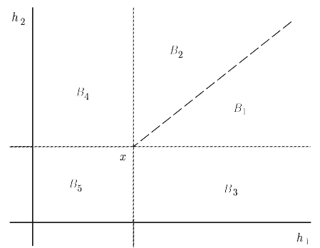
Fig. 1 Optimal basis regions of Example 1.

The optimal basis regions for the solution of this problem are illustrated in Figure 1.

Here, the optimal bases are B

corresponding to (y

) , B

corresponding to

) , B

corresponding to (y

−

) , B

corresponding to (y

−

) ,and B

corresponding to (y

−

) with dual multipliers

=(1, 0)

=(0, 1)

(1,−1)

=(−1,1)

,and

=(−1,−1)

, respectively. Figure 1 shows the

regions in which each of these bases is optimal.

We let p

= P(

) for i = 3,4,5 . To make the calculations somewhat sim-

pler, we divide

and

into two sections each depending on x as

(x)+

(x) and

(x)+

(x) where

(x)={

∈

≤

(

) ≤x

+min(1−x

,1−x

)},

(x)={

∈

+min(1−x

,1−x

) <

(

) ≤ 1},

(x)={

∈

≤ h

(

) ≤ x

+ min(1 −x

,1 −x

)},and

(x)={

∈

+ min(1 −x

,1 −x

) < h

(

) ≤ 1} with corresponding

integrals of h over each of these regions given by

(x) ,

(x) ,and

(x) respectively. In this way,

(x) and

(x) are symmetric around the di-

agonal x

= x

with one of

(x) and

(x) corresponding to a rectangular

region of positive probability if 1 ≥x

> x

or 1 ≥ x

> x

With these deﬁnitions, we can then write Q(x) for Example 1 as

Q(x)=

∑

i=1

∑

j= 0

(

(x) −Tx)+

∑

i=3

(

(x) −Tx). (1.6)

Finding the value of

h for each region then yields the following expression

(Exercise 2):

8.1 Direct Solutions with Multiple Integration 345

Q(x)=

+ x

−4x

+ x

+ 2(1 −x

)

max[0,−x

+ x

]

+max[0,x

−x

](2(1 −x

)

(min[1−x

,1 −x

])

for any x ∈ [0,1]

The regions

are polyhedral (Exercise 4) in general, which, as in Example

1, yields direct integration procedures when these regions are simple enough to

have explicit integration formulas. Unfortunately, this is not often the case for the

regions that are common in stochastic programs with recourse. As Exercise 2

demonstrates, even in the simple cases of uniform distributions, the expectations

over different regions depends on the relative values of the components of x and

may require signiﬁcant computation to ﬁnd exactly.

In problems with probabilistic constraints, however, there are possibilities for

creating deterministic equivalents when the data are, for example, normal as in

Theorem 3.18. In general, however, efﬁcient computation requires some form of

approximation.

In the following sections, we explore several methods for approximating the

value function and its subgradient in stochastic programming. The basic approaches

are either approximations with known error bounds or approximations based on

Monte Carlo procedures that may have associated conﬁdence intervals. In the re-

mainder of this chapter and Chapter 10, we explore bounding approaches, while in

Chapter 9 we also consider methods based on sampling.

Exercises

1. The principle of Gaussian quadrature is to ﬁnd points and weights on those

points that yield the correct integral over all polynomials of a certain degree.

For example, we can solve for points,

, and weights, p

, p

,sothat

we have a probability ( p

+ p

= 1 ) and distribution that matches the mean,

( p

+ p

), the second moment, ( p

+ p

(2)

), and the third

moment, ( p

+ p

(3)

). Solve this for a uniform distribution on [0, 1]

to yield the two points, 0.211 and 0.788 , each with probability 0.5.

(a) Verify that this distribution matches the expectation of any polynomial up

to degree three over [0,1] .

(b) Consider a piecewise linear function, f , with two linear pieces and 0 ≤

f (

) ≤ 1for0≤

≤ 1 . How large a relative error can the Gaussian

quadrature points give? Can you use two other points that are better?

2. Derive the expression of Q(x) for Example 1 in (1.7)using(1.6).

3. Verify that Q(x) for Example 1 is convex on [0,1]

using (1.7).

4. Show that each region

is polyhedral.

346 8 Evaluating and Approximating Expectations

8.2 Discrete Bounding Approximations

The most common procedures in stochastic programming approximations are to ﬁnd

some relatively low cardinality discrete set of realizations that somehow represents

a good approximation of the true underlying distribution or whatever is known about

this distribution. The basic procedures are extensions of Jensen’s inequality ([1906],

generalization of the midpoint approximation) and an inequality due to Edmundson

[1956] and Madansky [1959], the Edmundson-Madansky inequality, a generaliza-

tion of the trapezoidal approximation. For convex functions in

, Jensen provides

a lower bound while Edmundson-Madansky provides an upper bound. Signiﬁcant

reﬁnements of these bounds appear in Huang, Ziemba, and Ben-Tal [1977], Kall

and Stoyan [1982] and Frauendorfer [1988b].

We refer to a general integrand g(x, ξ) . Our goal is to bound E(g(x)) =

[g(x,ξ)] =



g(x,ξ)P(dξ) . The basic ideas are to partition the support

into

a number of different regions (analogous to intervals in one-dimensional integra-

tion) and to apply bounds in each of those regions. We let the partition of

= {S

,l = 1,...,

}.Deﬁne

= E[ξ | S

] and p

= P[ξ ∈ S

] . The basic

lower bounding result is the following.

Theorem 1. Suppose that g(x,·) is convex for all x ∈D.Then

E(g(x)) ≥

∑

l=1

g(x,

) . (2.1)

Proof: Write E(g(x)) as

E(g(x)) =

∑

l=1



g(x,ξ)P(dξ)

∑

l=1

E[g(x, ξ) | S

]

≥

∑

l=1

g(x,E[ξ | S

]) , (2.2)

where the last inequality follows from Jensen’s inequality that the expectation of a

convex function of some argument is always greater than or equal to the function

evaluated at the expectation of its argument, i.e., E(g(ξ)) ≥ g(E(ξ)) (see Exer-

cise 1).

This result applies directly to approximating Q(x) by Q

(x)=

∑

l=1

Q(x,

) . The approximating distribution P

is the discrete distribution with

atoms, i.e., points

of probability p

> 0forl = 1,...,

. By choosing S

so that each S

∈ S

is completely contained in some S



∈ S

, the approxi-

mations actually improve, i.e.,

8.2 Discrete Bounding Approximations 347

E(g(x)) ≥ E

(g(x)) ≥ E

(g(x)) . (2.3)

Various methods can achieve convergence in distribution of the P

to P .Anex-

ample is given in Exercise 2.

In general, the goal of reﬁning the partition from

+ 1 is to achieve as

great an improvement as possible. We will describe the basic approaches; more

details appear in Birge and Wets [1986], Frauendorfer and Kall [1988], and Birge

and Wallace [1986]. Three basic decisions are to choose the cell, S

∗

∈ S

,in

which to make the partition, to choose the direction in which to split S

∗

,andto

choose the point at which to make the split.

The reader should note that this section contains notation speciﬁc to bounding

procedures. To keep the notation manageable, we reuse some from previous sec-

tions, including a and b for endpoints of rectangular regions and c for points

within these intervals at which to subdivide the region. For ease of exposition,

suppose that the sets S

are all rectangular, deﬁned by [a

] × ···× [a

] .

The most basic reﬁnement scheme for l =

∗

is to ﬁnd i

∗

and c

∗

so that

(

) splits into S

(

+ 1)=[a

] ×...[a

∗

] ×[a

] and S

(

+ 1)=

] ×...[c

∗

] ×[a

] .

If we also have an upper bound UB(S

) ≥ E[g(x,

) |

∈ S

] for each cell

, then the most likely choice for S

∗

is the cell that maximizes p

(UB(S

) −

g(x,

)) , which bounds the error attributable to the approximation on S

. Reduc-

ing this greatest partition error appears to offer the most hope in reducing the error

on the

+ 1 approximation.

The direction choice is less clear. The general idea is to choose a direction in

which the function g is “most nonlinear”. The use of subgradient (dual price)

information for this process was discussed in Birge and Wets [1986]. Frauendor-

fer and Kall [1988] improved on this and reported good results by considering

all 2

m+1

pairs, (

) , of vertices of S

,where

,...,a

,...,

) and

,...,b

,...,

) with

= a

or b

.Given x , they assume a dual vector,

,at Q(x,

) and

at Q(x,

) . Because these represent subgradients of the

recourse function Q(x, ·) ,wehave Q(x,

) −(Q(x,

(

−

)) =

≥ 0

and Q(x,

)−(Q(x,

(

−

)) =

≥0 . They then choose k

∗

that max-

imizes min{

} over k .Theylet i

∗

be i such that

∗

and

∗

differ in the

i th coordinate. The position c

∗

is then chosen so that Q(x,

∗

−b

∗

Q(x,

∗

−a

∗

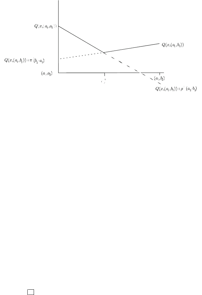
) . (See Figure 2, where we use

for the subgradient at

) and

for the subgradient at (a

) .) The general idea is then to choose

the direction that yields the maximum of the minimum of linearization errors in each

direction.

Reﬁnement schemes clearly depend on having upper bounds available. These

bounds are generally based on convexity properties of g and the ability to obtain

each

in terms of the extreme points. The fundamental result is the following

theorem that also appears in Birge and Wets [1986]. In the following, we use P as

themeasureon

instead of

because we wish to obtain a different measure

derived from this domain. In context, this change should not cause confusion. We

348 8 Evaluating and Approximating Expectations

Fig. 2 Choosing the direction according to the maximum of the minimum linearization errors.

also let ext

be the set of extreme points of co

and E is a Borel ﬁeld of ext

in this case, the collections of all subsets of ext

Theorem 2. Suppose that

→g(x,

) is convex and

is compact. For all

∈

let

(ξ,·) be a probability measure on (ext

,E ) , such that



e∈ext

(ξ,de)=ξ , (2.4)

and

→

(

),A) is measurable for all A ∈ E .Then

E(g(x)) ≤



e∈ext

g(x,e)

(de) , (2.5)

where

is the probability measure on E deﬁned by

(A)=



(

),A)P(d

) . (2.6)

Proof: Because g is convex in

,for

g(x,

) ≤



e∈ext

g(x,e)

(

,de) . (2.7)

Substituting

(

) for

and integrating with respect to P , the result in (2.5)is

obtained.

This result states that if we can choose the appropriate

and ﬁnd

, we can

produce an upper bound. The key is to make the calculation of

as simple as pos-

sible. Of course, the cardinality of ext

may also play a role in the computability

of the bound.

8.2 Discrete Bounding Approximations 349

One way to reduce the cardinality of the supporting extreme points is simply to

choose the extreme point that has the highest value as an upper bound. Let this up-

per bound be UB

max

(x)=sup

e∈ext

g(x,e) ≥



e∈ext

g(x,e)

(de) ≥ E(g(x)) from

Theorem 2, regardless of the particular

. While UB

max

may only involve a single

extreme point, it is often a poor bound (see the result from Exercise 3). Its calcu-

lation also often involves evaluating all the extreme points to maximize the convex

function g(x,·) .

In general, bounds built on the result in Theorem 2 construct the probability

measure

so that each extreme point e

has some weight, p

) .

The following bounds, described in more detail in Birge and Wets [1986], ﬁnd these

weights in various cases. The ﬁrst is general but involves some optimization. The

second involves simplicial regions, and the third uses rectangular regions.

Because

is constructed to be consistent with the distribution of ξ ,wemust

have that



(

)P(d



e∈ext

(

),de)P(d

)



e∈ext



(

),de)P(d

)



e∈ext

(de) . (2.8)

Hence,

∈P = {

is a probability measure on E ,and E

[e]=

}. The next

upper bound, originally suggested by Madansky [1960] and extended by Gassmann

and Ziemba [1986], builds on this idea by ﬁnding an upper bound through a linear

program to maximize the objective expectation over all probability measures in P .

We write this bound as UB

mean

,where

mean

(x)= max

,...,p

∑

k=1

g(x,e

)

s. t.

∑

k=1

∑

k=1

= 1 , p

≥ 0 , k = 1,...,K .

(2.9)

As we shall see in Section 8.5, the probability measure that optimizes the linear pro-

gram in (2.9) is the solution of a moment problem in which only the ﬁrst moment

is known. Another interpretation of this bound is that it represents the worst pos-

sible outcome if only the mean of the random variable is known. Optimizing with

this bound, therefore, brings some form of risk avoidance if no other distribution

information is available.

Assuming that the dimension of co

is N , Carath´eodory’s theorem states that

must be expressable as a convex combination of at most N + 1 points in ext

Finding these N +1 points may, however,again involve computationsfor the values

350 8 Evaluating and Approximating Expectations

at all extreme points. The number of extreme point representations may be much

higher than N + 1if

is, for example, rectangular, but lower if, for example,

is a simplex, i.e., a convex combination of N + 1 points,

, i = 1,...,N + 1,such

that

−

are linearly independent for i > 1 . The representation of interior points

is, in fact, unique. Indeed, the p

in this case are called the barycentric coordinates

Although

may not be simplicial itself, it is often possible to extend Q(x,·)

from

to some simplex

including

. The bound obtained with this approach

is written UB

. In this bound, the number of points used in the evaluation remains

one more than the dimension of the afﬁne hull of

. Frauendorfer [1989, 1992]

gives more details about this form of approximation and various methods for its

reﬁnement.

Often,

is given as a rectangular region. In this case, the number of extreme

points is 2

. The number of simplices containing

may also be exponential in

N . With relatively complete information about the correlations among random vari-

ables, however, bounds can be obtained that assign the same weight to each extreme

point of

(or a rectangular enclosing region), regardless of the value of x .This

attribute is quite beneﬁcial in algorithms where x may change frequently as an

optimal solution is sought.

The basic bounds for rectangular regions follow Edmundson and Madansky, for

which, the name Edmundson-Madansky (E-M) bound is used. They begin with the

trapezoidal type of approximation on an interval. Here, if

=[a,b] , we can easily

construct

(

,·) in Theorem 2 as

(

,a)=

(

) and

(

,b)=1 −

(

) ,where

(

b−

b−a

. Integrating over

, we obtain

(a)=



(

),a)P(d

)



b −

(

)

b −a

P(d

)

b −

b −a

. (2.10)

We then also have

(b)=

−a

b−a

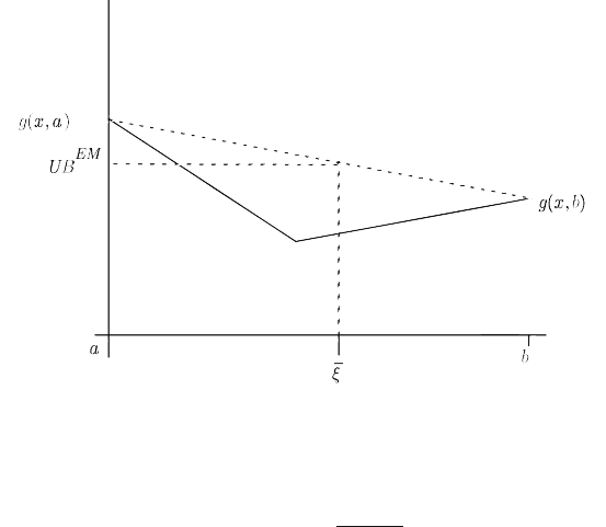
. The bound obtained is UB

(x)=

(a)g(x,a)+

(b)g(x,b) ≥ E(g(x)) . Observe in Figure 3 that this bound represents approximat-

ing the integrand g(x,·) with the values formed as convex combinations of extreme

point values. This is the same procedure as in trapezoidal approximation for nu-

merical integration except that the endpoint weights may change for nonuniform

probability distributions.

The E −M bound on an interval extends easily to multiple dimensions, where

=[a

]×···×[a

] if either g(x,·) is separable in the components of

,in

which case, the bound is applied in each component separately, or the components

of ξ are stochastically independent. In this case, the bound is developed in each

component i = 1toN in order so that the full independent

bound contains the

product of all combinations of each interval bound, i.e.,

8.2 Discrete Bounding Approximations 351

Fig. 3 Example of the Edmundson-Madansky bound on an interval.

EM−I

(x)=

∑

e∈ext



∏

i=1

−e

−a



g(x,e) , (2.11)

where

is again assumed polyhedral.

Example 1 (continued)

We return again to Example 1 and suppose an initial solution, ¯x =(0.3,0.3)

.From

(1.7), Q( ¯x)=0.466 . Our initial lower bound using the mean of the random vector

is then the Jensen lower bound, LB

= Q( ¯x,

h =(0.5,0.5)

)=0.2.

The upper bounds can be found using the values at the extreme points of

the support of h . These values are Q( ¯x,(0, 0)

)=0.6, Q( ¯x,(0,1)

)=1.0,

Q( ¯x, (1,0)

)=1.0, and Q(¯x,(1,1)

)=0.7. For UB

max

( ¯x) ,wemusttakethe

highest of these values; hence, UB

max

( ¯x)=1.0. For UB

mean

, notice that

h =

(1/2)(1, 0)

+(1/2)(0, 1)

;so,UB

mean

( ¯x)=UB

max

( ¯x)=1.0.For UB

, each

extreme point is weighted equally, so UB

( ¯x)=(1/4)(1 + 1 + .7 + .6)=0.825 .

For the simplicial approximation, let

= co{(0,0),(2,0),(0,2)} , which includes

the support of h . In this case, the weights on the extreme points are

(0,0)=0.5

and

(2,0)=

(0,2)=0.25 . The resulting upper bound is UB

( ¯x)=0.5(.6)+

0.25(2)(2)=1.3.

To reﬁne the bounds, we consider the dual multipliers at each extreme point.

At (0,0) ,theyare (−1, −1) .At (1, 0) ,theyare (1,−1) .At (0,1) ,theyare

(−1,1) .At (1,1) , both bases B

and B

are optimal, so the multipliers are (0,1) ,

(1,0) , or any convex combination. The linearization along the line segment from

352 8 Evaluating and Approximating Expectations

(0,0) to (1,0) is the minimum of Q( ¯x,(1,0)

)−Q( ¯x,(0,0)

)+(−1,−1)

(1,0)=

1−(0.6−1)=1.4andQ( ¯x,(0,0)

)−Q( ¯x, (1,0)

)+(1,−1)

(−1,0)=0.6−(1−

1)=0.6 . Hence, the minimum error on (0, 0) to (1,0) is 0.6 . Similarly, for (0,0)

to (0,1) , the error is 0.6.From (1,0) to (1,1) , the minimum error is 0.3ifthe

(0,1) subgradient is used at (1,1) ; however, the minimum error on (0,1) to (1,1)

is then min{1 −(0.7 −1),0.7−(1

−1)}= 0.7 . Thus, the maximum of these errors

over each edge of the region is 0.7 for the edge (0,1) to (1,1) .

To ﬁnd the value of c

∗

to split the interval [a

= 0,b

= 1] , we need to ﬁnd

where Q( ¯x,(0,1)

)−c

∗

= Q( ¯x,(1, 1)

)+(c

∗

−1) or where 1−c

∗

= 0.7−1+ c

∗

i.e., where c

∗

= 0.65 . We obtain two regions, S

=[0,0.65] ×[0, 1] and S

[0.65,1] ×[0,1] , with p

= 0.65 and p

= 0.35 .

The Jensen lower bound is now LB

= 0.65(Q( ¯x,(0.325, 0.5)

))+

(0.35)(Q( ¯x,(0.825, 0.5)

)) = 0.65(0.2)+0.35(0.525)=0.31375 . The

upper bounds are UB

max

( ¯x)=0.65(1)+0.35(1)=1, UB

mean

( ¯x)=0.65(0.5)(1 +

0.65)+0.35(0.5)(1 + 0.7)=0.83375 , and UB

( ¯x)=0.65(0.25)(1 + 0.7 +

0.65 + 0.6)+0.35(0.25)(0.7 + 0.7 + 1 + .65)=0.74625 . (The simplicial bound

is not given because we have split the region into rectangular parts.) Exercise 3 asks

for these computations to continue until the lower and upper bounds are within 10%

of each other.

Exercises

1. For Example 1, ¯x =(0.1, 0.7)

, compute Q( ¯x) , the Jensen lower bound, and

the upper bounds, UB

mean

, UB

max

, UB

,and UB

2. Prove Jensen’s inequality, E(g(ξ)) ≥ g(E(ξ)) , by taking an expectation of the

points on a supporting hyperplane to g(ξ) at g(E(ξ)) .

3. Follow the splitting rules for Example 1 until the Edmundson-Madansky upper

and Jensen lower bounds are within 10% of each other. Compare UB

max

on each step.

8.3 Using Bounds in Algorithms

The bounds in Section 8.2 can be used in algorithms in a variety of ways. We de-

scribe three basic procedures in this section: (1) uses of lower bounds in the L -

shaped method with stopping criteria provided by upper bounds; (2) uses of upper

bounds in generalized programming with stopping rules given by lower bounds; and

(3) uses of the dual formulation in the separable convex hull function. The ﬁrst two

approaches are described in Birge [1983] while the last is taken from Birge and Wets

[1989].

The L -shaped method as described in Chapter 5 is based on iteratively providing

a lower bound on the recourse objective, Q(x) . If a lower bound, Q

(x) ,isused

8.3 Using Bounds in Algorithms 353

in place of Q(x) , then clearly for any supports, E

x + e

,if Q

(x) ≥ E

x + e

Q(x) ≥ E

x + e

. Thus, any cuts generated on a lower bounding approximation of

Q(x) remain valid throughout a procedure that reﬁnes that lower bounding approx-

imation. This observation leads to the following algorithm. We suppose that Q

(x)

and Q

(x) are approximating lower and upper bounding approximations such that

lim

j→∞

(x)=Q(x) and lim

j→∞

(x)=Q(x) . We suppose that P

is the

j th lower bounding approximation measure so that Q

(x)=



(x,ξ)P

) .

To simplify the algorithm in the following, we assume that all feasibility cuts are

generated separately in (3.2) below before the sequential bounding procedure be-

gins (which generally can be accomplished by ﬁrst considering all extreme points

of the domain of the random variables).

L -Shaped Method with Sequential Bounding Approximations

Step 0.Set r = s = v = k = 0.

Step 1.Set

+ 1 . Solve the linear program (3.1)–(3.3):

min z = c

x +

s. t. Ax = b , (3.1)



x ≥d



,= 1,...,r , (3.2)



x +

≥ e



,= 1,...,s , (3.3)

x ≥ 0 ,

∈ ℜ .

Let (x

) be an optimal solution. If no constraint (3.3)ispresent,

is set equal

to −∞ and is ignored in the computation.

Step 2.Find Q



,ξ)P

) ,the j th lower bounding approxima-

tion. Suppose −(

(ξ))

T ∈

∂

,ξ) (the simplex multipliers associated with

the optimal solution of the recourse problem). Deﬁne

s+1



(

(ξ))

) (3.4)

and e

s+1



(

(ξ))

) . (3.5)

Let w

= e

s+1

−E

s+1

= Q

). If

≥ w

, x

is optimal, relative to the

lower bound; go to Step 4. Otherwise, set s = s + 1 and return to Step 1.

Step 3.Find Q



,ξ)P

(

) ,the j th upper bounding approxima-

tion. If

≥ Q

) , stop; x

is optimal. Otherwise, reﬁne the lower and upper

bounding approximations from

+ 1.Let

+ 1.GotoStep2.