Buede D.M. The Engineering Design of Systems Models and Methods
Подождите немного. Документ загружается.

(5) there is a proper value function defined at the value node (i.e., one that is
defined over all the nodes with arcs into the value node); and (6) there are
proper functions defined for each deterministic node. An influence diagram that
is well formed can be evaluated analytically to determine the optimal decision
strategy implied by the structural, functional, and numerical definition of the
influence diagram. The analytic operations needed to evaluate an influence
diagram numerically are evidence absorption, deterministic absorption, null
reversal, arc reversal, and deterministic propagation [Shachter, 1986].
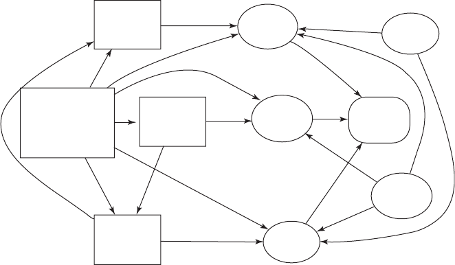
The influence diagram in Figure 13.9 shows an example of an influence
diagram for a requirements allocation decision for the design of a new elevator
system. The systems engineer is considering the use of one of two new
technologies (power or controller); the large decision node (center left of
Figure 13.9) defines the three alternatives. The requirements allocati on (shown
as three separate decision nodes) of costs, performance, and availability will be
different if one or neither of these technologies is included in the design. Since
this initial decision will be known when the three requirements allocation
decisions are made, there are arcs from the initial decision node to the three
requirements allocation decision nodes. The other arcs between the three
requirements allocation decision nodes indicate the order in which the decisions
will be made: performance, availability, and cost. (The decision maker is free to
select any order among these three nodes.) These allocations and the prior
uncertainty of the systems engineering team about the power and controller
technologies will affect the uncerta inty about the elevator’s cost, performance,
and availability. The arcs between the chance nodes are identical to those
shown in Figure 13.5. Note, this diagram shows the uncertainty of elevator
Cost
Requirements
Allocation
Elevator
System Cost
Power
Technology
Elevator Operational
Architecture:
1) Hi Tech Control
2) Hi Tech Power
3) Low Risk
Performance
Requirements
Allocation
Elevator
Performance
Fundamental
Objective
Availability
Requirements
Allocation
Elevator
Availability
Controller
Technology
FIGURE 13.9 Sample influence diagram for requirements allocation.
13.5 UNCERTAINTY IN DECISIONS 423
performance to be independent of power technology. In this simplified
example, the fundamental objective is comprised of three elements: cost,
performance, and availability.
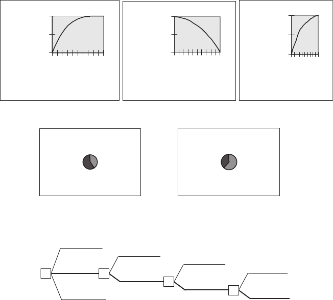
The results of a case study analysis of the above elevator architecture and
requirements allocation decision are shown in Figure 13.10. First, the value
functions for elevator performance (an index of various passenger waiting times),
life-cycle cost, and availability and their weights are shown. Note that marginal
decreasing returns to scale is shown in each curve as capability moves from
the minimum acceptable threshold to the technological maximum. Next, the
uncertainties associated with the two technologies in question are shown.
The other uncertainties encoded as part of the analysis are not shown here.
The analytical results show that the allocated architecture and the requirements
allocation associated with the advanced power technology should be chosen to
be consistent with the requirements (the value structure captured by the trade-off
Summary of Elevator Case Study
Value Functions
Weights:
0.5 0.3 0.2
0
50
100
0.3
0.6
0.9
1.2
Performance
Value
0
50
100
2.2
3
3.8
Life Cycle Cost
Value
0
50
100
0.8
0.88
0.95
Availability
Value
Technology Uncertainties
Controller Technology Power Technology
Status
Quo
60%
Success
40%
Success
60%
Status
Quo
40%
Risk Analysis Results
Control 57
Control 44
Control 55
Power 59 Control 45
Power 59
Power 59
Low Risk 45
Power 59
Operational
Architecture
Performance
Allocation
Availability
Allocation
Cost
Allocation
FIGURE 13.10 Summary of requirements allocation case study.
424
DECISION ANALYSIS FOR DESIGN TRADES
requirements) and the uncertainty about the technologies. The alternative
associated with the control technology is very close; in fact, too close to be
confident that the power technology is preferred given the limitations of value
and probabilistic assessments. The low-risk alternative is clearly inferior;
the design team could feel comfortable choosing either of the new technologies.
The choice of technology would significantly change the requirements allocation
decisions made in the three subsequent decision nodes.
13.5.4 Risk Preference and Expected Utility
Webster’s dictionary defines risk simply as the ‘‘exposure to the chance of loss,’’
and most people have at least an intuitive sense of what risk means to them. But
from a decision-making perspective, it is essential to provide a more formal
definition. The Defense Systems Management College (DSMC), [1989] in their
Risk Management Handbook, defines risk as ‘‘the combination of the prob-
ability of an eve nt occurring and the significance of the consequence of the
event occurring’’ and defines risk management as ‘‘the various processes used to
manage risk.’’
There are several strategies used for dealing with risk: avoidance, transfer-
ence, managem ent, and analysis. Risk avoidance is the selection of the low-risk
alternative; unfortunately, what seems to be low risk intuitively is high risk in
some cases. For example, consider a situation in which you have a sizable
portfolio of U.S.-based stocks and are considering purchasing either another
U.S. stock or what is consider ed a high-risk international stock. The interna-
tional stock is often the lower risk alternative because its perfor mance is either
negatively correlated or uncorrelated with the performance of your portfolio
while the performance of the low-risk U.S. stock is highly correlated with your
current portfolio.
Risk transference involves options that transfer risk to others, an example
being the purchase of insurance. The insurance purchaser is willing to pay a
fixed price and have the insurance company take the risk of a major loss.
Risk management involves the use of hedging strategies; a hedging strategy is
the maintenan ce of fallback options in case a riskier option fails. The failure is
not catastrophic because the fall back option can be used. This is common in
systems engineering when multiple contractors are asked to develop the same
component; one contractor is pursuing the high-risk and high-performance
approach that will be used if successful, while another contractor is pursuing a
more conservative approach.
Risk analysis addresses risk explicitly when decisions are made in uncertain
situations. Addressing the uncertainty faced in a decision by assigning
probabilities to the uncertain outcomes, producing a lottery, has been discussed
above. If the outcomes are measured on a numerical scale (e.g., dollars) that
captures the value associated with the outcome, the expected value of the
lottery is used as a measure of the attractiveness of the lottery. However, if the
outcomes of the lottery are substantial compared to the wealth or well being of
13.5 UNCERTAINTY IN DECISIONS 425

the decision maker, the expected value may not be an appropriate measure of
the value of the lott ery, as judged by many decision makers. The value
associated with a lottery is called the certain equivalent, the value the decision
maker would be willing to accept in place of the lottery. Since this notion of
certain equivalence is a subjective judgment that is special to the individual (or
set of stakeholders) and the context at the time of the decision, a mathematical
description of risk preference must be guided by the feelings of decision makers.
A utility or risk preference function, u, is intr oduced to be a function of the
outcome values of the lottery. If such a function exists, the inverse functi on of
the expected utility of the lottery is the value of the certain equivalent of the
lottery that can then be used to compare the attractiveness of the lottery with
other lotteries. For example, consider the two lotteries in Figure 13.11 in which
the outcomes are measured in dollar s. The expected values (EV) of these two
lotteries are:
EVð1Þ¼0:5 $1000 þ 0:5 $ 0 ¼ $500
EVð2Þ¼0:1 $100;000 þ 0:9 $10;000 ¼ $1000
These expected values indicate that lottery 2 is preferred to lottery 1;
EV(2)WEV(1). Yet many people, who cannot afford a loss of $10,000, would
prefer the first lottery with the lower expected value. In other words, for those
people, the expected utility of lottery 1Wthe expected utility of lottery 2, or
0:5uð$1000Þþ0:5uð$0Þ40:1u ð$100;000Þþ0:9uð$10;000Þð13:12Þ
Mathematically, if the inverse function of u(.) exists, then Eq. (13.12) can be
restated as
u
1
½0:5uð500Þþ0:5uð0Þ4u
1
½0:1uð100;000Þþ0:9uð10;000Þ ð13:13Þ
The question is: ‘‘Will such a function generally explain the decision maker’s
risk preference judgments over all possible lotteries?’’ The two expressions on
.5
.5
$1000
$0
.1
.9
$100,000
-$10,000
Win
Lose
Win
Lose
FIGURE 13.11 Comparison of two lotteries.
426
DECISION ANALYSIS FOR DESIGN TRADES
either side of the inequality in Eq. (13.13) are called the certain equivalents of
the two lotteries.
The risk premium, x
p
, of a lottery is defined to be the difference between the
expected value of the lottery and the certain equivalent,
~
x,
x
p
¼
x
~
x ð13:14Þ
For risk-averse decision makers the certain equivalent will always be less than
the expected value and the risk premium will be positive.
13.5.4.1 Assessing A Risk Preference Function. Discussion of a risk pre-
ference function for a specific decision assumes that the outcomes of the
decision have been characterized by a value function that collapses all
dimensions of value onto one dimension, commonly called the numeraire. A
money equivalent is the most common numeraire, but others are also possible.
The risk preference function is then a function over the value numeraire.
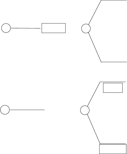
There are two types of questions involving a certain equivalent and a two-
outcome lottery that one can ask a decision maker during a risk assessment
session. These two questi on types are shown in Figure 13.12. The first question
type assumes the probabilities of the lottery are known and the decision maker
.5
.5
$10
0
$0
1
? = $35
Query about the certain
equivalent given a completely
defined lottery.
? = .6
1 - ? = .4
$100
$0
1
$35
Query about the probability
of a lottery given all outcomes
are completely defined.
=
=
FIGURE 13.12 Simple risk preference assessment queries.
13.5 UNCERTAINTY IN DECISIONS 427
is asked to provide one of the outcome values, typically the value of the certain
equivalent. However, one could fix the certain equivalent and ask for the value
of either the best outcome or worst outcome. The second question assumes that
all of the outcome values are known, including the certain equivalent, and the
decision maker is asked to supply the probability value.
Unfortunately, research has shown that people do not provide coherent
answers to these two types of queries. That is, in general the answers to the
second question type are going to suggest much greater risk aversion than
answers by the same individual to the first question type. A not uncommon
response to the first query, which has an expected value of $50, is $35, yielding a
risk premium of $15. Now if $35 is the certain equivalent in the second query,
an individual might respond that the question mark for the probability of $100
in the second lottery would be 0.6. The risk premium for this second lottery is
$25 (the expected value of $60 minus the certainty equivalent of $35).
The first question type is asking directly for the response that will be
substituted into various analyses. Therefore, it is somewhat more appropriate
to ask this question. However, very few decision makers have thought seriously
about these issues in general, and even fewer have thought about them with
respect to a specific decision situation. The assessment process is therefore a
learning experience for the decision maker. The responses to the early questions
should be treated as a warm-up process.
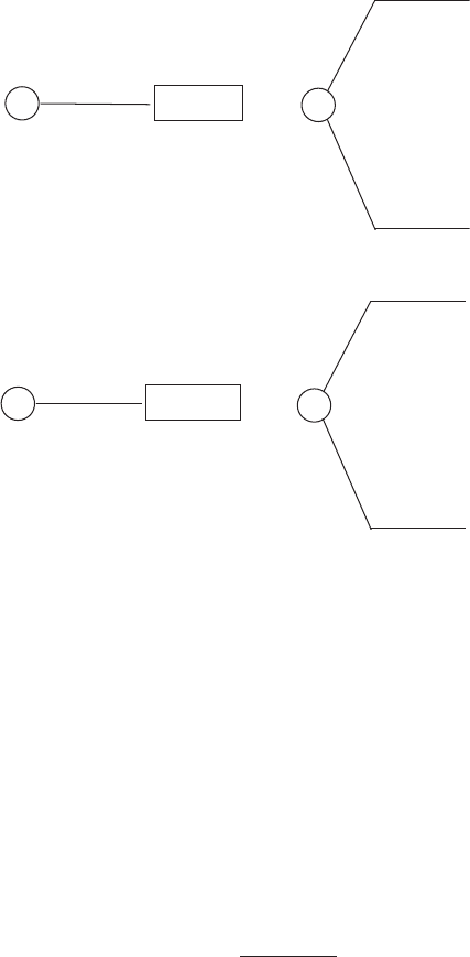
A second caution for the risk assessment process is that there is a very
substantial zero effect. That is, people exhibit risk-averse behavior for gains but
risk-seeking behavior for losses. Figure 13.13 shows responses for a certainty
equivalent that demonstrates this behavior. The risk premium is $15 for the top
lottery and $15 for the bottom lottery. The risk-averse person in the top
lottery would have a certain equivalent of less than $50 for the bottom lottery.
Generally, people do not want to exhibit this ‘‘zero effect’’ once the seeming
contradiction is pointed out to them and will switch to a consistent risk-averse
(or risk-seeking) policy.
To investigate the decision maker’s risk preference fully in the region of
outcomes associated with the current decision, multiple lottery questions
should be asked in this region. For illustrative purposes, suppose the decision
involves gains of up to $10,000 and losses as great as $10,000. We arbitrarily set
the end points of the utility scale as u($0) = 0 and u($10,000) = 1. Figure 13.14
provides six such lotteries and the responses of the decision maker shown in the
boxes. Note that the utilities shown under each figure are calculated as in the
following example:
uð$2;500Þ¼:5 uð$10;000Þþ:5 uð$0Þ
¼ :5 ð1Þþ:5 ð0Þ
¼ :5
Figure 13.15 displays the resulting risk preference function. Note the decreasing
rate of increase associated with this curve, mathematically known as a concave
428 DECISION ANALYSIS FOR DESIGN TRADES
curve. A risk-neutral decision maker would have a straight line as a risk
preference function ; risk-seeking behavior is typified by a convex curve.
13.5.4.2 Exponential Risk Preference. Define the risk aversion coefficient
g ¼u
00
ðxÞ=u
0
ðxÞ.Ifg is a constant, it can be sho wn by simple integration that
the risk preference function must take the form
uðxÞ¼
k
1
x þk
2
; if g ¼ 0
k
1
e
gx
þk
2
; if g =2 0
(
ð13:15Þ
A common way to write such a risk preference function is
uðxÞ¼
1 e
gx
1 e
gx
max
; ð13:16Þ
where x
max
is the largest value that x is expected to take. Thus , for any valued
outcome x, the utility of x can be calculated using the exponential utility
function. Note that this format produces
uðx
max
Þ¼1:0
uð0Þ¼0
.5
.5
$100
$0
1
? = $35
.5
.5
$0
-$100
1
=
=
? = -$35
FIGURE 13.13 Illustration of the zero effect.
13.5 UNCERTAINTY IN DECISIONS 429
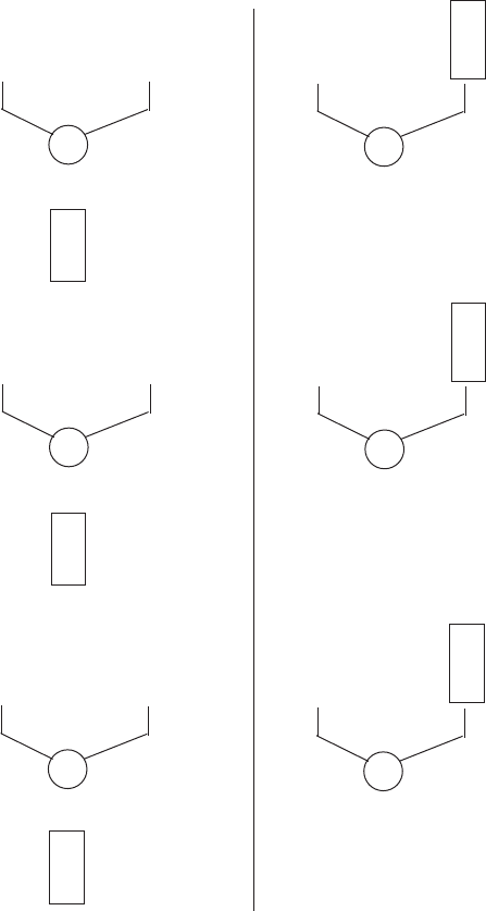
.5
.5
$10,000
$0
$2500
=
.5
.5
$2500
$0
$1000
=
.5
.5
$10,000
$2500
$5000
=
u(0) = 0 u(10,000) = 1
u(2500) = .5 u(1000) = .25 u(5000) = .75
.5
.5
$10,000
$0
-$2600
=
.5
.5
$0
-$4200
-$2600
=
.5
.5
$0
-$6200
-$4200
=
u(-2600) = -1 u(-4200) = -2 u(-6200) = -4
Query 1 Query 2 Query 3
Query 4 Query 5 Query 6
FIGURE 13.14 Assessment queries for risk preference function.
430

The risk preference function plotted in Figure 13.15 is an exponential risk
preference function with g = 0.00025.
Another important concept in risk preference is the risk tolerance, or the
inverse of the risk aversion coefficient. For the exponential risk preference
function and its co nstant risk aversion coefficient, the risk tolerance is constant.
In Figure 13.15, the risk tolerance is $4000. For an expected value decision
maker the risk aversion coefficient is zero, making the risk tolerance infinity.
The exponential risk preference function has another very special property,
called the delta property This property is stated as follows: An increase in all
outcomes of the lottery by a constant amount, D, results in an increase of the
certain equivalent by the same amount, A. So, for example, in the first example
above suppose that the certain equivalent for fifty — fifty gamble of $100 and
$0 was $35. Now, if each prize is increased by $100 and the certain equivalent of
a fifty — fifty gamble on $200 and $100 becomes $135, then the delta property is
satisfied for at least this one case. The exponential risk preference function is
the only function that can satisfy this property.
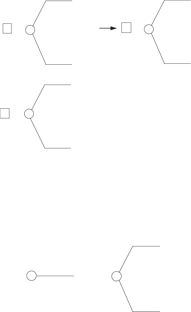
One very important implication of the delta property is that the buying and
selling prices of a lottery are the same. For example, the maximum that a
decision maker was willing to pay, B. for a lottery is the amount that when
subtracted by every outcome made us indifferent to having the lottery and not
having it, or a value of $0. Similarly, the minimum that the decision maker
would sell the lottery for, S, is its certain equivalent; also see Figure 13.16. If the
risk preference function is exponential, it can be proven that B=Sthrough the
use of the delta property. For other risk preference functions the buying and
selling prices of a lottery are not necessarily equal.
There is a ‘‘quick and dirty’’ method for assessing a decision maker’s risk
aversion coefficient for an exponential utility function. The value of R for
which the decision maker is indifferent to accepting the lottery in Figure 13.17
x
u(x)
-5
-4
-3
-2
-1
0
1
-10000 -5000
0
5000
10000
FIGURE 13.15 Assessed risk preference points.
13.5 UNCERTAINTY IN DECISIONS 431
is the risk tolerance. That is, the certainty equivalent of the lottery in Figure
13.17 is 0 when R is the risk tolerance of the decision maker. It can be shown
that g = 1/R.
The exponential risk preference function is used as an approximation early
in risk analyses to determine the effect of risk preference on the choice of
alternatives. If this choice is sensitive in the appropriate region of the decision
maker’s risk tolerance, then more detailed analysis of the decision maker’s risk
preference is appropriate.
.5
.5
$x - B
$y - B
0
.5
.5
$x
$y
=
=
S
.5
.5
$
x
$y
B
=
adding B to
the certain equivalent
and each outcome
So B = S.
FIGURE 13.16 Buying and selling prices are equal for exponential risk preference.
0.5
0.5
R
-R/
2
1
0 =
FIGURE 13.17 Risk aversion coefficient lottery.
432
DECISION ANALYSIS FOR DESIGN TRADES