Caers J. Modeling Uncertainty in the Earth Sciences
Подождите немного. Документ загружается.


P1: OTA/XYZ P2: ABC
JWST061-09 JWST061-Caers April 6, 2011 13:24 Printer Name: Yet to Come
9.3 VISUALIZING UNCERTAINTY 161
Figure 9.5 Location of a few selected Earth models.
Euclidea
n
distance
high
low
Connecvit
y
distance
Contaminan
t
arrival
me
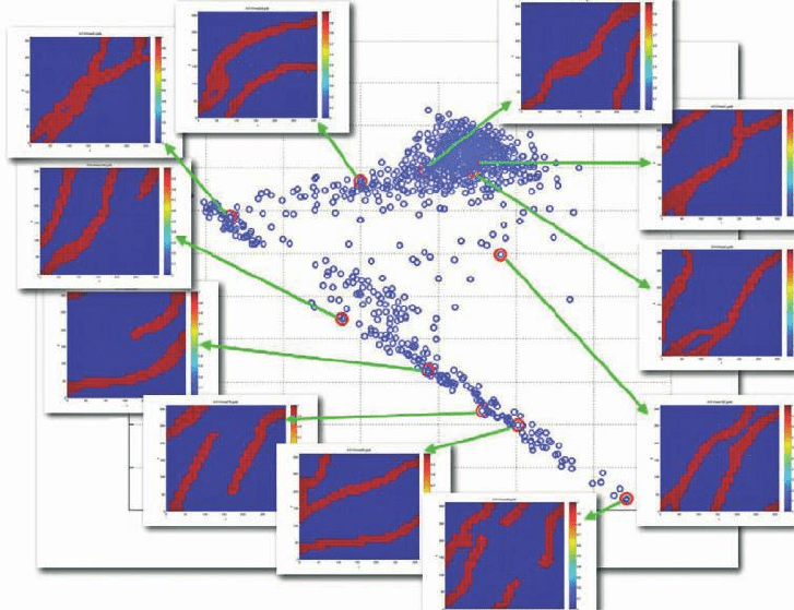
Figure 9.6 Plotting a response function (arrival time) at locations of models projected with
different distances.
P1: OTA/XYZ P2: ABC
JWST061-09 JWST061-Caers April 6, 2011 13:24 Printer Name: Yet to Come
162 CH 9 VISUALIZING UNCERTAINTY
9.3.2 Determining the Dimension of Projection
In all of the above examples, Earth models were plotted in 2D, simply because it is easy to
visualize a distribution of points in 2D. Consider another case, shown in Figure 9.7. One
thousand Earth models are created, each showing a distribution of channel ribbons. Some
of the Earth models as well as their 2D MDS projection are shown in Figure 9.6. The dis-
tance used is again a difference in measure of connectivity between any two Earth mod-
els. The connectivity is measured from the bottom-left corner of the grid to the top-right
corner. Clearly models that plot on the left-hand side of Figure 9.6 are well connected.
How good is this projection? In other words, is the Euclidean distance between any two
points in this 2D plot a good approximation of the difference in connectivity? This can
be assessed by plotting the Euclidean distances between any two Earth models versus
the difference in connectivity. This plot will contain 1000 × 1000 points (Figure 9.8,
left). It seems that for small distances, there is still some discrepancy. We can therefore
decide to plot models in 3D, as shown in Figure 9.8 (middle). Figure 9.9 compares 2D
and 3D MDS of the same Earth models with the same connectivity distance defined be-
tween them. The correlation improves, and will continue to improve by increasing the
dimension (five dimensions seems accurate enough; Figure 9.8, right).
Figure 9.7 Ribbon-like Earth models and their 2D MDS projection.

P1: OTA/XYZ P2: ABC
JWST061-09 JWST061-Caers April 6, 2011 13:24 Printer Name: Yet to Come
9.3 VISUALIZING UNCERTAINTY 163
2D map 3D map 5D map
3
2.5
2
1.5
0.5
0
1
2D Euclidean distance
3
2.5
2
1.5
0.5
0
1
3D Euclidean distance
Connecvity difference
Connecvity difference
0 0.5 1 1.5 2 2.5 3
0
0.5 1 1.5 2 2.5 3
3
2.5
2
1.5
0.5
0
1
5D Euclidean distance
Connecvity difference
0
0.5 1 1.5 2 2.5 3
Figure 9.8 Plotting the Euclidean distance of 2D, 3D and 5D projection versus the connectivity
difference.
9.3.3 Kernels and Feature Space
Defining a distance on Earth models and projecting them in a low dimensional (2D or
3D) Cartesian space presents a simple but powerful diagnostic on model variability in
terms of the application at hand, at least if the chosen distance is reflective of the dif-
ference in studied response. Clearly, how model uncertainty is looked at is application
dependent (see the difference between Figures 9.2 and 9.3). In Chapter 10, these plots
will be used to select a few Earth models that are representative for the entire set (for
target response uncertainty evaluation) and to assess what parameters are most influenc-
ing the response (sensitivity or effect analysis). However, as shown in Figure 9.9, the
cloud of models in a 2D or 3D projection Cartesian space may have a complex shape,
making the selection of representative models (as done Chapter 10) difficult. In computer
science kernel techniques are used to transform from one metric space into a new metric
space such that, after projecting in 2D, 3D and so on, the cloud of models displays a
simpler arrangement.
Figure 9.9 A 2D and 3D MDS map of the Earth models shown in Figure 9.6. The color indicates
the connectivity of each model (blue = low, red = high).
P1: OTA/XYZ P2: ABC
JWST061-09 JWST061-Caers April 6, 2011 13:24 Printer Name: Yet to Come
164 CH 9 VISUALIZING UNCERTAINTY
Metric
Spac
e
on
x
N
o
Axis
defined
MDS
Feature
S
pac
e
on
x
N
o
Axis
defined
MDS
ϕ
ϕ
-1
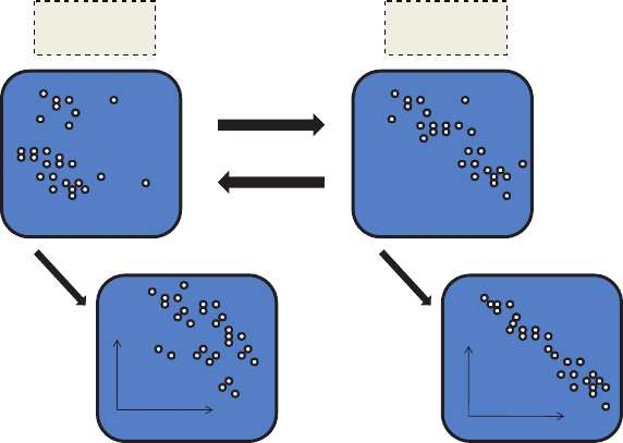
Figure 9.10 Concept of metric and feature space and their projection with MDS.
The goal, therefore, is to transform (change) the Earth models such that they arrange
in simpler fashion in the MDS plot. To achieve this, consider an Earth model x
i
and its
transformation using some multivariate function :
x
i
→ (x
i
)or
⎛
⎜
⎝
x
1
.
.
.
x
L
⎞
⎟
⎠
→
⎛
⎜
⎝
(x
1
)
.
.
.
(x
L
)
⎞
⎟
⎠
Figure 9.10 depicts what is happening.
What is this function ? Consider what we are trying to achieve (Figure 9.10). We
would like for the cloud of points, such as in Figure 9.9, to be simpler, maybe by stretch-
ing it out more. We also know that this cloud of points is uniquely (up to rotation, trans-
lation and reflection) quantified by knowing the distance between any two x
i
. Hence, in
order to change this cloud, we do not need to change the x
i
individually, we only need to
transform the distances between the x
i
, and, as a consequence, in order to rearrange the
cloud we do not need a function to change x
i
but a function that changes the distances
between them. This is good news, because x is of very large dimension (N) and finding
such a multivariate function may be hard, while the distance is a simple scalar and there
are only L × L distances to transform. A function that transforms distances or trans-
forms from one metric (or distance) space to another is termed in the technical literature
a kernel function. In other words, a kernel is also a distance of sorts (or measures of dis-
similarity, but technically mathematicians call it a dot-product; the values of matrix B in
Equation 9.5 are also dot-products). There are many kernel functions (as there are many

P1: OTA/XYZ P2: ABC
JWST061-09 JWST061-Caers April 6, 2011 13:24 Printer Name: Yet to Come
9.3 VISUALIZING UNCERTAINTY 165
distances and dot-products); we will just discuss one that is convenient here, namely the
radial basis kernel (RBF), which in all generality is given by:
K
ij
= k(x
i
, x
j
) = exp
−
(x
i
− x
j
)
T
(x
i
− x
j
)
2
2
Note that this RBF is function (a single scalar) of two Earth models x
i
and x
j
and of
parameter , called the bandwidth, which needs to be chosen by the modeler. The band-
width acts like a scalar of length. If is very large, then K
ij
will be zero except when
i = j, meaning that all x
i
tend to be very dissimilar; while if is close to zero, then all x
i
are deemed very similar. So it is necessary to choose a that is representative of the differ-
ence between the various x
i
. Practitioners have found that choosing the bandwidth equal
to the standard deviation of values in the L × L distance matrix is a reasonable choice.
Note that the RBF is function of the Euclidean distance (x
i
− x
j
)
T
(x
i
− x
j
). We want
to make this RBF kernel a bit more general, that is, by making it function of any distance,
not just the Euclidean distance. This can be done simply by means of MDS as follows:
1 Specify any distance d(x
i
, x
j
).
2 Use MDS to plot the locations in a low dimension (e.g., 2D or 3D), call these locations
x
d,i
and x
d, j
with d the dimension of the MDS plot.
3 Calculate the Euclidean distance between x
d,i
and x
d, j
.
4 Calculate the kernel function with given .
K
ij
= k(x
i
, x
j
) = exp
−
(x
d,i
− x
d, j
)
T
(x
d,i
− x
d, j
)
2
2
Since we have a new indicator of “distance,” namely K
ij
, we also have a new “metric
space’, which is traditionally called the “feature space” (Figure 9.6). Now, the same MDS
operation can be applied to matrix K. The eigenvalue decomposition of K is calculated
and projections can be mapped in any dimension (Figure 9.9), for example in 2D using
f =2
= V
K, f =2
1/2
K, f =2
where V
K, f =2
contains the eigenvectors of K belonging to the two largest eigenvalues
of K contained in the diagonal matrix
K, f =2
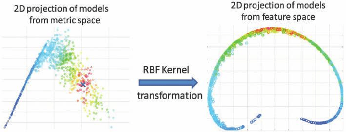
. An illustrative example is provided in
Figure 9.11. One thousand Earth models were mapped into 2D Cartesian space (the same
as Figure 9.6). Shown on the right-hand side of Figure 9.11 are the 2D projections of
models in feature space. Note how the complex cloud of Earth model locations has be-
come more “stretched out” (left-hand side). In the next chapter we will see that this gives
way to better model selection and quantification of response uncertainty.
P1: OTA/XYZ P2: ABC
JWST061-09 JWST061-Caers April 6, 2011 13:24 Printer Name: Yet to Come
166 CH 9 VISUALIZING UNCERTAINTY
Figure 9.11 Comparison of locations of models and response function evaluation after projec-
tion with MDS from metric space and feature space.
9.3.4 Visualizing the Data–Model Relationship
The above application of MDS demonstrates how the possibly complex uncertainty rep-
resented by many alternative Earth models can be visualized through simple 2D or 3D
scatter plots. In many applications, data are used to constrain models of uncertainty, as
was discussed in Chapters 7 and 8. In other applications, new data become available over
time and the current model of uncertainty needs to be updated. In a Bayesian context this
means that the current “posterior,” that is, the current set of models matching the data as
well as reflecting the current prior information available, now become the “new prior.”
It is, therefore, of considerable interest to study the relationship between any prior
model of uncertainty and the data available. In Chapter 7 it was discussed that there may
be a conflict between the prior and the data–model relationship (the likelihood), since
they are often specified by different modelers. Can a simple plot be created, therefore,
comparing the prior model uncertainty with the data?
To illustrate that this is indeed possible, consider a realistic case example. A synthetic
but realistic reservoir case study, known as the “Brugge data set,” named after the Flemish
town where the conference involving this data set was held, is used as demonstration. As
prior uncertainty, a number of input modeling parameters are unknown:
r
The models are either binary rock types (sand vs background) each with different per-
meability and porosity characteristics or the system is directly modeled using the conti-
nuous permeability and porosity variables. In either case, spatial uncertainty is present.
r
The geological scenario is uncertain: either the system contains sand fluvial chan-
nel objects within a background (binary) or the (binary) system was modeled using
variogram-based techniques. However, the Boolean model was taken as deterministic,
so was the variogram.
r
The proportion of the sand rock type in the reservoir is uncertain with given probability
distribution.
P1: OTA/XYZ P2: ABC
JWST061-09 JWST061-Caers April 6, 2011 13:24 Printer Name: Yet to Come
9.3 VISUALIZING UNCERTAINTY 167
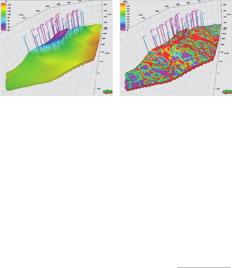
Figure 9.12 Pressure obtained by forward simulation (left), An example Earth model, the red
color indicates channel sands, the purple indicates more shaly rocks (right).
An example Earth models is shown in Figure 9.12. All models are constrained to some
“hard data,” which are available from the wells drilled in the reservoir. These models
represent the prior uncertainty.
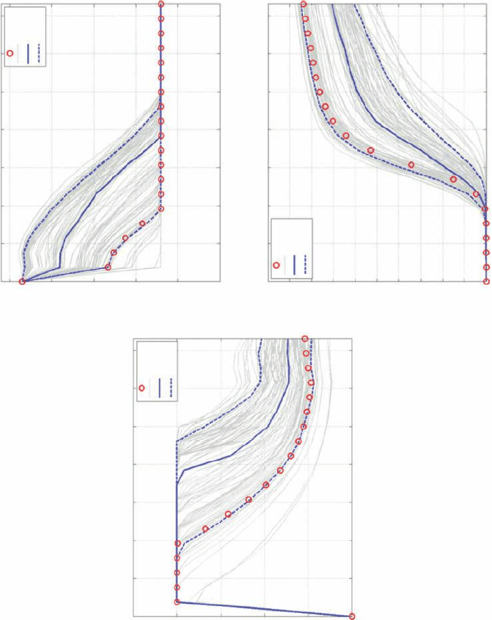
The field data concern the historical monthly values of water rate, oil rate and pres-
sure measurements in 20 producing wells over a 10 year period. The forward model is a
(finite difference) simulation model of flow in the subsurface. The initial and boundary
conditions are assumed known, as are many of the fluid properties. Figure 9.12 shows
the pressure variation in this reservoir obtained by forward simulation on the model
on the left.
To visualize prior uncertainty as well as the historical production data we proceed as
follows. Firstly, apply the forward model g to each of the L Earth models m
i
, resulting
in a forward model response g
i
= g(m
i
), which is a vector containing the time series
production responses of oil/water rate and pressure. Figure 9.13 shows these responses
for one of the 20 producing wells. As distance simply define some distance between the
forward model responses for each of the models:
d(m
i
, m
j
) = d
g
(g(m
i
), g(m
j
)) for example d
g
(g(m
i
), g(m
j
)) =
(g
i
− g
j
)
T
(g
i
− g
j
))
In addition, we have the real data from the actual field, which we term d. In fact, these
data can be seen as the response from the “true” Earth m
true
d = g(m
true
)
if we assume that the forward model reflects correctly the Earth’s response and an Earth
model m captures the true Earth realistically. This means that we can also calculate the
P1: OTA/XYZ P2: ABC
JWST061-09 JWST061-Caers April 6, 2011 13:24 Printer Name: Yet to Come
168 CH 9 VISUALIZING UNCERTAINTY
Data
Inial
p
50
p
50
and p
90
Data
Inial
p
50
p
50
and
p
90
Data
Inial
p
50
p
50
and
p
90
0
0
500
Well watercut, fracon
1000 1500 2000
TIME, days
2500 3000 3500
Well oil producon rates, sm
3
/day
0
0
500
500
1000
1000
1500
1500
2000
2000
TIME, days
2500 3000
2500
3500
Well boom hole pressure, psia
0
0
500
500
1000
1000
1500
1500
2000
2000
TIME, days
2500 3000
2500
3500
0.1
0.2
0.3
0.4
0.5
0.6
0.7
0.8
0.9
1
Figure 9.13 Oil production rate over time (left), well-bore pressure (top right), fraction of production that is water (bottom right).
P1: OTA/XYZ P2: ABC
JWST061-09 JWST061-Caers April 6, 2011 13:24 Printer Name: Yet to Come
9.3 VISUALIZING UNCERTAINTY 169
distance between the responses of the models m
i
and the true Earth as represented by the
data, namely:
d
g
(g(m
i
), d) =
(g
i
− d)
T
(g
i
− d)
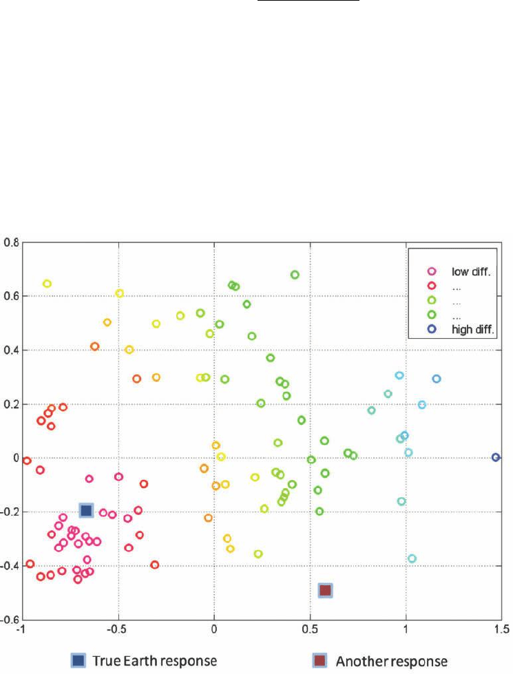
This means that we have an L + 1 (L Earth models and 1 true Earth) distance matrix
that allows plotting, using MDS, the L models as well as the true Earth. Figure 9.14 shows
the result for the Brugge data set. One observes that in this case, the “true Earth” (or better
its response) plots with the various alternative prior Earth models. This is good news: it
means that the modeling effort at least captures what the true unknown is, in terms of
this specific response. Should the true Earth plot be outside of this scatter of points, as
is hypothetically shown in Figure 9.14, then either the prior uncertainty is incorrect, the
data are incorrect or the data–model relationship is incorrect. Such evaluation is important
Figure 9.14 MDS plot of the response of 65 Earth models as well the response from the true
Earth (field data). The color indicates the difference (diff.) in response with the field data.
P1: OTA/XYZ P2: ABC
JWST061-09 JWST061-Caers April 6, 2011 13:24 Printer Name: Yet to Come
170 CH 9 VISUALIZING UNCERTAINTY
before addressing the issue of integrating these data into the Earth models, for example
using inverse modeling techniques as discussed in Chapter 7.
Further Reading
Borg, I. and Groenen, P. (1997) Modern Multidimensional Scaling: Theory and Applications, Springer,
New York.
Peters, L., Arts, R.J., Brouwer, G.K. et al. (2010) Results of the Brugge benchmark study for flooding
optimization and history matching. SPE Reservoir Evaluation & Engineering, 13(3), 391–405. SPE-
119094-PA. doi: 10.2118/119094-PA.
Sch
¨
oelkopf, B. and Smola, A. (2002) Learning with Kernels, MIT Press, Cambridge, MA.