Caers J. Modeling Uncertainty in the Earth Sciences
Подождите немного. Документ загружается.

P1: OTA/XYZ P2: ABC
JWST061-08 JWST061-Caers March 29, 2011 10:31 Printer Name: Yet to Come
FURTHER READING 151
Further Reading
Bond, C.E., Gibbs, A.D., Shipton, Z.K., and Jones, S. (2007) What do you think this is? “Conceptual
Uncertainty” in geoscience interpretation. GSA Today, 17, 4–10.
Caumon, G. (2010) Towards stochastic time-varying geological modeling. Mathematical Geosciences,
42(5), 555–569.
Cherpeau, N., Caumon, G., and Levy, B. (2010). Stochastic simulation of fault networks from 2D seis-
mic lines. SEG Expanded Abstracts, 29, 2366–2370.
Holden, L., Mostad, P., Nielsen, B.F., et al. (2003) Stochastic structural modeling. Mathematical Geol-
ogy, 35(8), 899–914.
Suzuki, S., Caumon, G., and Caers, J. (2008) Dynamic data integration into structural modeling: model
screening approach using a distance-based model parameterization. Computational Geosciences, 12,
105–119.
Thore, P., Shtuka, A., Lecour, M., et al. (2002) Structural uncertainties: Determination, management,
and applications. Geophysics, 67, 840–852.
P1: OTA/XYZ P2: ABC
JWST061-08 JWST061-Caers March 29, 2011 10:31 Printer Name: Yet to Come
P1: OTA/XYZ P2: ABC
JWST061-09 JWST061-Caers April 6, 2011 13:24 Printer Name: Yet to Come
9
Visualizing Uncertainty
We cannot process hundreds of models in climate modeling when we know one such model
may take several days of computing time. We cannot run flow simulation on thousands of
reservoir models to evaluate whether drilling a new well is worth the cost. The good news
is that we don’t have to. We can be selective of the models that we use to process. However, this
requires that we get a better visual insight in the uncertainty represented by those thousands
of models and in this chapter some important tools to do so are discussed.
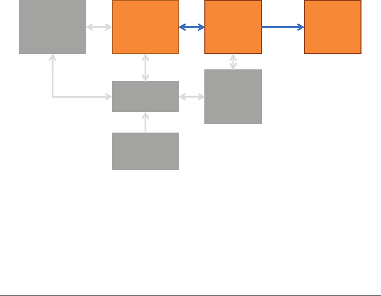
Physical
model
Spaal
Stochasc
model
Spaal
Input
parameters
Forecast
and
decision
model
Physical
input
parameters
Raw
observaons
Data sets
response
uncertain
uncertain
certain or uncertainuncertain
uncertain/error
uncertain
uncertain
9.1 Introduction
The purpose of Earth modeling and prediction is very clear: produce forecasts (climate,
reservoir flow, contaminant transport, groundwater recharge efficiency), estimate reserves
(mineral resources, total contaminated sediment volume) or make decisions (choose
where to drill well, decide whether to obtain more data, decide to clean up, change
Modeling Uncertainty in the Earth Sciences, First Edition. Jef Caers.
© 2011 John Wiley & Sons, Ltd. Published 2011 by John Wiley & Sons, Ltd.
153
P1: OTA/XYZ P2: ABC
JWST061-09 JWST061-Caers April 6, 2011 13:24 Printer Name: Yet to Come
154 CH 9 VISUALIZING UNCERTAINTY
policies). As observed so far, many fields of expertise in modeling are required to com-
plete this task: spatial modeling, structural modeling, process modeling, geological inter-
pretation, data processing and interpretation, modeling of partial differential equations,
inverse modeling, decision theory, and so on. In many applications, a rigorous assess-
ment of uncertainty is critical since it is fundamental to any geo-engineering decision
making process.
In this book several techniques to model uncertainty about the Earth’s properties and
structures have been discussed. We saw how we can represent such uncertainty by gener-
ating many alternative Earth models, possibly hundreds or thousands. Now what do we do
with them? How do we start incorporating them into a decision making process? How do
we process them for prediction purposes? Regarding the last question, the term “applying
a transfer function” has been coined for taking a single model and calculating a desired
or “target” response from it. If many Earth models have been created, the transfer func-
tion needs to be applied to each Earth model, resulting in a set of alternative responses
that model/reflect the uncertainty of the target response. This is a common Monte Carlo
approach. In a reservoir/aquifer context, this response may be the amount of water or
oil from a new well location; in mining this could be a mining plan obtained through
running an optimization code; in environmental applications this may be the amount of
contaminant in a drinking water well; in climate models the sea temperature change at
a specified location, the carbon dioxide build up in the atmosphere over time. Based on
this response prediction various actions can be taken or certain decisions made. Either
more data is gathered with the aim of further reducing uncertainty towards the decision
goal or controls are imposed on the system (pumping rates, control valves, carbon diox-
ide reduction) or decisions are made (e.g., policy changes, clean up or not). The problem
often is that processing hundreds of alternative Earth models may become too demanding
CPU-wise. We cannot process hundreds of models in climate modeling when we know
one such model may take several days of computing time. We cannot run flow simulation
on thousands of reservoir models to evaluate whether drilling a new well is worth the
cost. It would be extremely tedious to include hundreds of models into decision problems
and decision trees such as those presented in Chapter 4. The good news is that we don’t
have to. We can be selective of the models that we use to process. However, this requires
that a better visual insight is obtained into the uncertainty represented by those thousands
of models and in this chapter some important tools to do so are discussed.
9.2 The Concept of Distance
An observation critically important to understanding the uncertainty puzzle is that the
complexity and dimensionality (number of variables) of the input data and models are
far greater than the complexity and dimensionality of the desired target response. In fact,
the desired output response can be as simple as a binary decision question: do we drill or
not, do we clean up or not? At the same time the complexity of the input model can be
enormous, containing complex relationships between different types of variables, physics
(e.g., flow in porous media or wave equations) and is, moreover, varying in a spatially
complex way. For example, if three variables (soil type, permeability and porosity) are
P1: OTA/XYZ P2: ABC
JWST061-09 JWST061-Caers April 6, 2011 13:24 Printer Name: Yet to Come
9.2 THE CONCEPT OF DISTANCE 155
simulated on a one million cell grid and what is needed is contaminant concentration at
10 years for a groundwater well located at coordinate (x,y), then a single input model has
dimension of 3 × 10
6
while the target response is a single variable.
This simple but key observation suggests that the uncertainty represented by a set of
Earth models can be represented in a simpler way, if the purpose of these Earth mod-
els is taken into account. Indeed, many factors may affect contaminant concentration at
10 years to a varying degree of importance. If a difference in value of a single input vari-
able (porosity at location (x,y,z)) leads to a considerable difference in the target response,
then that variable is critical to the decision making process. Note that the previous state-
ment contains the notion of a “distance” (a difference of sorts). However, because Earth
models are of large dimension, complex and spatially/time varying, it may not be trivial
to discern variables that are critical to the decision making process easily. To make the
uncertainty puzzle simpler, the concept of a distance is introduced. A distance is a single,
evidently positive value that quantifies the difference between any two “objects.” In our
case the objects are two Earth models. If there are L Earth models, then a table of L × L
distances can be specified. The mathematical literature offers many distances to choose
from; a very common distance that is introduce later is the Euclidean distance (in 2D it
would be a measure of the distance between two geographic locations on a flat plane).
The choice between distances provides an opportunity to choose a distance that is related
to the response differences between models. This will allow “structuring” uncertainty
with a particular response in mind and create better insight into what uncertainty affects
the response most. Earth models can be considered as puzzle pieces: if two puzzle pieces
are deemed similar then they can be grouped and represented by some average puzzle
piece (the sky, the grass, etc.). This, however, requires a definition of similarity. This is
where the distance comes in. In making that distance a function of the desired response,
the grouping becomes effective for the decision problem or response uncertainty question
we are trying to address. For example, if contaminant transport from a source to a specific
location is the target, then a distance measuring the connectivity difference (from source
to well) between any two Earth models would be a suitable distance.
Defined in the next section are some basic concepts related to distances that allow the
uncertainty represented by a large variety of models to be analyzed very rapidly. As an
initial illustration of how a distance renders complex phenomena more simple, consider
the example in Figure 9.1. As discussed in Chapter 8, uncertainty in structural geometry
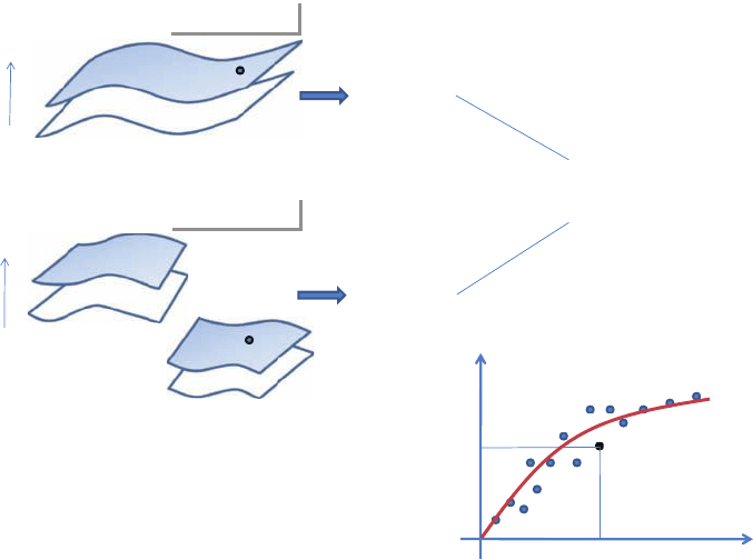
is complex and attributed to various sources. Figure 9.2 shows a few structural models
from a case study whereby a total of 400 structural Earth models are built. As discussed
in Chapter 8, a structural model consists of horizon surfaces cut by faults. To distinguish
between any two structural models, the joint difference between corresponding surfaces
in a structural model is then used as a distance, termed d
H.
Figure 9.1 explains how this is
done exactly. A surface consists of points x,y with a certain depth z (at least for surfaces
of non-overhang structures). The joint distance between these depth values z for each
surface of a model k and the same surface of a model is then a measure of the difference
in structural model. How this distance is actually calculated is not the point of discussion
for this book. Figure 9.1 shows that such difference depends on the difference in fault
structures as well as the difference in horizons (as was outlined in Chapter 8).
P1: OTA/XYZ P2: ABC
JWST061-09 JWST061-Caers April 6, 2011 13:24 Printer Name: Yet to Come
156 CH 9 VISUALIZING UNCERTAINTY
z
z
Earth model k
Earth
model ℓ
(
x
i
,y
i
,z
ik
)
(
x
i
,y
i
,z
iℓ
)
d
H,k,
ℓ
=joint distance between z ’s and z
’s
k
ℓ
Response k
Resp
o
ns
e ℓ
d
H
Difference in
response
betwee
n
any two
models
Difference in
response
between models k
and ℓ
d
H,k,
ℓ
Difference in
response
between Earth models k
and ℓ
Figure 9.1 Calculating the difference between two structural models and comparing it with the
difference in response calculated from such models.
To evaluate whether this distance can actually provide a better insight into the differ-
ence in cumulative oil production response between any two models, the squared differ-
ence in response is also calculated and this difference plotted versus d
H
in Figure 9.1.
If this is done for all pairs of models and the moving average taken, the smooth line in
Figure 9.1 is obtained. Note that the latter plot is nothing more than the variogram of
production response, as defined in Chapter 5; however, the distance on the x-axis of this
variogram plot is the geometrical distance between any two models. Recall that the var-
iogram is a measure of dissimilarity, so small variogram values mean that samples close
by (in the distance defined) are related to each other. If the distance was not informative
about a difference in production response, then this variogram would be a pure nugget
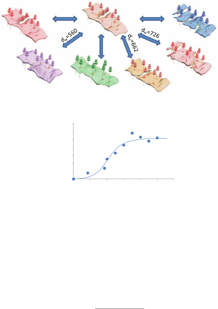
variogram. Clearly this is not the case, as shown in Figure 9.2, for the actual case. The
distance is informative about production response difference and provides a way to struc-
ture variability between a set of complex structural models in a simple fashion.
9.3 Visualizing Uncertainty
9.3.1 Distances, Metric Space and Multidimensional Scaling
The notion of distance can now be put in a more mathematical context. The equations are
given here for completion; what is important, however, are the plots that result from them.
P1: OTA/XYZ P2: ABC
JWST061-09 JWST061-Caers April 6, 2011 13:24 Printer Name: Yet to Come
9.3 VISUALIZING UNCERTAINTY 157
d
H
=115
d
H
=636
d
H
=876
Averag
e square difference in response
b
etwee
n any
two
models
0
0.2
0.4
0.6
0.8
1
1.2
1.4
120010008006004002000
Ha
u
ss
do
rf
d
ista
nce
d
H
Figure 9.2 Seven structural Earth models out of 400 are shown (top). The distance d
H
between
a single model and the other six is plotted; (bottom) the variogram of production response as
function of the distance d
H
.
A single (input) Earth model i is represented by a vector x
i
, which contains either
the list of properties (continuous or categorical or a mix of them) in each grid cell or an
exhaustive list of variables uniquely quantifying that model. The “size” or “dimension”
N of the model is then the length of this vector, for example, the number of grid cells in
a gridded model. N is typically very large. L denotes the number of alternative models
generated with typically L N. All models are collected in the matrix X:
X = [x
1
x
2
...x
L
]
T
of size L ×N (9.1)
One of the most studied distances is the Euclidean distance, which is defined as
d
ij
=
(x
i
− x
j
)
T
(x
i
− x
j
) (9.2)
if this distance were applied to a pair of models x
i
, x
j
. Mathematically, one states that
models exist within a Cartesian space D (a space defined by a Cartesian axis system) of
high dimension N, each axis in the Cartesian grid representing the value of a grid cell.

P1: OTA/XYZ P2: ABC
JWST061-09 JWST061-Caers April 6, 2011 13:24 Printer Name: Yet to Come
158 CH 9 VISUALIZING UNCERTAINTY
A distance, such as a Euclidean distance, defines a metric space M, which is a space
only equipped with a distance; hence it does not have any axis, origin, nor direction
as, for example, a Cartesian space has. This means that the location of any x in this
space cannot be uniquely defined, only how far each x
i
is from any other x
j
, since only
their mutual distances are known. Even though locations for x in M cannot be uniquely
defined, some mapping or projection of these points in a low dimensional Cartesian space
can, however, be presented. Indeed, knowing the distance table between a set of cities,
we can produce a 2D map of these cities, which are uniquely located on this map up
to rotation, reflection and translation. To construct such maps, a traditional statistical
technique termed multidimensional scaling (MDS) is employed. The MDS procedure
works as follows. The distances are centered such that the maps origin is 0. It can be
shown that this can be done by the following transformation of the distance d
ij
into a new
variable b
ij
,
b
ij
=−
1
2
d
2
ij
−
1
L
L
k=1
d
2
ik
−
1
L
L
l=1
d
2
lj
−
1
L
2
L
k=1
L
l=1
d
2
kl
This scalar expression can be represented in matrix form as follows. Firstly, construct
a matrix A containing the elements
a
ij
=−
1
2
d
2
ij
(9.3)
then, center this matrix as follows
B = HAH with H = I −
1
L
11
T
(9.4)
with 1 = [1 1 1 ...1]
T
a row of L ones, I, the identity matrix of dimension L. B can also
be written as:
B = (HX)(HX)
T
of size L ×L (9.5)
Consider now the eigenvalue decomposition of B as:
B = V
B
B
V
T
B
(9.6)
In our case, L N and the distance is Euclidean, hence all eigenvalues are posi-
tive. We can now reconstruct (map onto a location in Cartesian space) any x in X in any
dimension from a minimum of one dimension up to a maximum of L dimensions, by
considering that
B = (HX)(HX)
T
= V
B
B
V
T
B
⇒ X = V
B
1/2
B
⇒ X
d
= V
B,d
1/2
B,d
: X
MDS
→ X
d
(9.7)
if we take the d largest eigenvalues. V
B,d
contains the eigenvectors belonging to the d

P1: OTA/XYZ P2: ABC
JWST061-09 JWST061-Caers April 6, 2011 13:24 Printer Name: Yet to Come
9.3 VISUALIZING UNCERTAINTY 159
largest eigenvalues contained in the diagonal matrix
B,d
. The solution X
d
retained by
MDS is such that the mapped locations contained in the matrix
X
d
=
x
1,d
x
2,d
...x
L,d
T
have their centroid as origin and the axes are chosen as the principal axes of X (proof
not given here). The length of each vector x
i,d
is d, the chosen mapping dimension.
Traditional MDS was developed for Euclidean distances, but as an extension the same
operations can be done on any distance matrix.
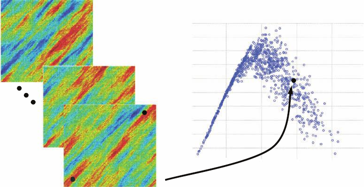
Consider the example illustrated in Figure 9.3. 1000 Earth models x
i
, i = 1,...,1000
are generated from a sequential Gaussian simulation (size N = 10 000 = 100 × 100; see
Chapter 7) using a spherical anisotropic variogram model and standard Gaussian his-
togram. The Euclidean distance is calculated between any two models resulting in a
1000 × 1000 distance matrix. A 2D mapping (d = 2) is retained of the Earth models
in Figure 9.3. What is important in this plot is that the (2D) Euclidean distance in Figure
9.2 is a good approximation of the (ND) Euclidean distance between the models. Each
point i in this plot has two coordinates which are equal to:
x
i,d=2
= (v
1,i
1
,v
2,i
2
)
with v
1,i
the i
th
entry of the first eigenvector. However, the actual axis values are not of
any relevance; it is the relative position of locations that matters because this reflects the
difference between the Earth models. So, in all of what follows in this book, any axis
-30
-25
-20
-15
-10
-5
0
5
10
15
20
-25 -20 -15 -10 -5 0 5 10 15 20
25
1000 Earth models
x
1
x
2
x
1000
Figure 9.3 1000 variogram-based Earth models and their locations after projection with MDS:
Euclidean distance case.
P1: OTA/XYZ P2: ABC
JWST061-09 JWST061-Caers April 6, 2011 13:24 Printer Name: Yet to Come
160 CH 9 VISUALIZING UNCERTAINTY
values are not shown in order to emphasize that only the relative location of points is
what matters. Notice how the cloud is centered around 0 = (0,0) as was achieved through
the centering operation above. Projecting models with MDS rarely requires dimensions
of five or higher such that the Euclidean distance between locations in the map created
with MDS correlates well with the actual distance specified.
Consider now an alternative distance definition between any two models. Using the
same models as previously, two points are located (A and B; Figure 9.4). A measure of
connectivity (the details of how this measure is exactly calculated are not given here)
is calculated for each Earth model. Such measure simply states how well the high val-
ues form a connected path between those two locations. The distance is then simply
the difference in connectivity between two models. Using this distance, we produce
an equivalent 2D map of the same models (Figure 9.4). Note the difference between
Figure 9.3 and Figure 9.4, although both plot locations of the same set of models. If the
connectivity-based projections (Figure 9.5) are investigated, it is noted how the Earth
models of the left-most group are disconnected (a lack of red color between location A
and B), while models on the right reflect connected ones. However, any two models that
map closely may look, at least by visual inspection, quite different.
Consider now the case where these models are used to assess uncertainty of a contam-
inant traveling from the source A to a well at location B. Suppose that we are interested
in the arrival time of such contaminant, then Figure 9.6 demonstrates clearly that a con-
nectivity distance nicely sorts models in a low dimensional space, while models projected
based on the Euclidean distance do not sort well at all. This will be important later, when
we attempt select Earth models based on travel times (or any other nonlinear response).
100
0
Earth
models
A
B
Figure 9.4 1000 Gaussian Earth models and their locations after projection with MDS: connec-
tivity distance case.