Crank J. Free and Moving Boundary Problems
Подождите немного. Документ загружается.

162
Analytical solutions
by-passed some
of
their complicated analysis.
The
minor errors
he
referred
to
are corrected in
the
above equations (personal communication
from K.S.). Soward also obtained results for
the
freezing of
the
terminal
cores of
both
sphere
and
cylinder by a new and simpler method based
on
a similarity variable.
Davis and
Hill (1982) developed a series solution of
the
sphere
problem after first using a boundary-fixing transformation.
4.
Front-tracking methods
4.1. Numerical techniques
FINITE-DIFFERENCE
methods have
been
used extensively for
the
numeri-
cal solution
of
moving boundary problems and, in recent years, finite-
element techniques have
been
introduced.
In
Ockendon and Hodgkins
(1975) accounts
by
Crank
(1975b)
and
by Fox (1975)
are
to
be
found.
More recent work is described in Wilson, Solomon, and Boggs (1978), by
Fox (1979),
and
by
Crank
(1981). Furzeland (1977a,1979a) surveys
many methods
and
presents
an
extensive bibliography.
In
a
later
paper
(1980)
he
examines a selection
of
methods for computational efficiency
and accuracy, programming complexity, and ease
of
generalization to
more
than
one
space dimension and to more complicated problems.
This chapter deals with numerical methods which compute, at each step
in
time,
the
position
of
the
moving boundary.
When
the
solution is
computed
at
points
on
a fixed grid in
the
space-time domain following
the
usual methods for obtaining a numerical solution
of
the
simple heat-flow
equation,
the
boundary
will
in general
be
between two grid points
at
any
given time. Therefore, special formulae
are
needed
to
cope with terms
like
au/ax
and
ds/dt, as well as with
the
partial differential equation itself,
in
the
neighbourhood
of
the
moving boundary. These formulae must
allow for unequal space intervals.
The
difficulty is compounded
if
implicit
finite-difference formulae
are
used, since
the
position of
the
moving
boundary is
not
known at
the
new time
and
some iterative procedure is
usually inevitable. Alternatively,
the
grid itself has
to
be
deformed in
some way,
or
some
transformation
of
variables adopted, so
that
the
moving boundary is always
on
a grid line
or
is fixed
in
the
transformed
domain.
An
early
paper
on
finite elements (Fisher and Medland 1974)
used special averaging procedures in
the
element containing
the
moving
boundary.
4.2.
Fixed
finite-diflerence grid
Suppose
the
heat-flow equation is
to
be
solved by using finite-
difference replacements for
the
derivatives in
order
to
compute values
of
temperature,
U;j'
at
discrete points
(i
8x,
j 8t)
on
a fixed grid in
the
(x,
t)
164
Front-tracking methods
plane.
At
any time j
8t,
the
phase-change boundary will usually
be
located
between two neighbouring grid points, say
i
8x
and
(i
+
1)
8x.
This can
be
allowed for by using modified finite-difference formulae which incorpo-
rate unequal space intervals
near
the
moving boundary. Interpolation
formulae of Lagrangian type can
be
used (Crank 1957a). Confining
attention
to
three-point formulae, we have for
the
general function
f(x)
which takes known values f(o.o),
f(al),
f(a0
at
the
three points x =
ao,
at>
a2
respectively
2
f(x)
= L
Hx)f(llj),
(4.1)
j=O
where
D(
)
P2(X)
~I
x
(x
-
llj)p~(llj)'
and
p~(llj)
is its derivative with respect
to
x at x =
llj.
It
follows
that
where
df
dx
= tb(x)f(ao) +
t~(x)f(al)
+
t~(x)f(a0,
tb(x)=
(X-al)(X-a;)
(ao-
al)(aO-
a0'
and similarly for
tHx),
t~(x).
Furthermore,
.!
d
2
f =
f(o.o)
+
f(al)
+
f(a;)
2
dx
2
(ao-al)(o.o-a0
(al-a;)(al-aO)
(a2-aO)(a2-al)"
(4.2)
(4.3)
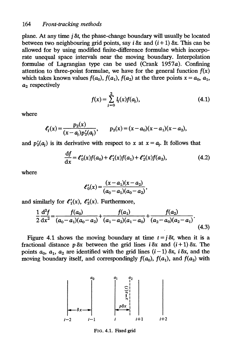
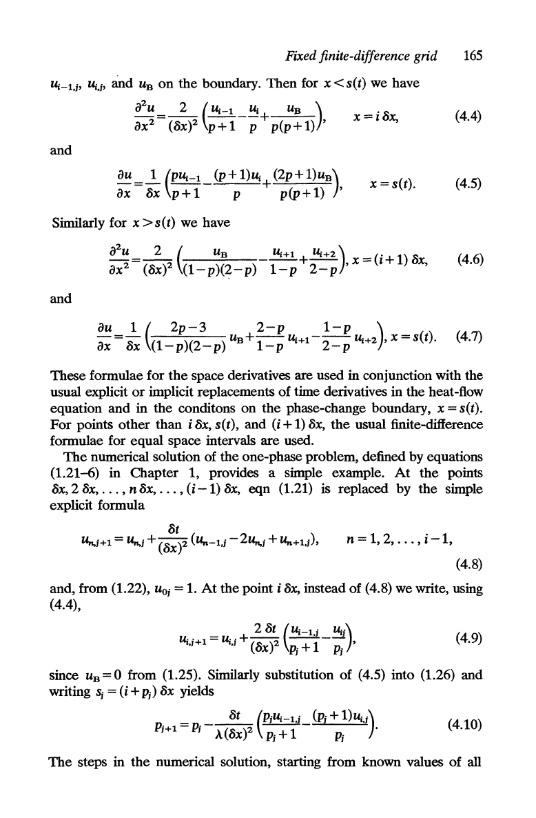
Figure 4.1 shows
the
moving boundary
at
time t = j
8t,
when it is a
fractional distance P
8x between
the
grid lines i 8x
and
(i
+
1)
8x.
The
points
ao,
at>
a2
are
identified with
the
grid lines
(i
-1)
8x,
i
8x,
and
the
moving boundary itself,
and
correspondingly f(o.o),
f(al),
and
f(a0
with
l,xJ
i-2
i-I
al
f2
r
~,
~:
I ,
><,
pax :
FIG. 4.1. Fixed grid
HI
H2
Fixed finite-difference grid
U;-l,j,
U;,j'
and
UB
on
the
boundary.
Then
for x < s(t) we have
and
iJ
2
u 2 ( U;-l
U;
UB)
-=--
----+
x=i8x,
iJx
2
(8X)2
p+1
P
p(p+1)
,
iJu
=~
(PU;-l_
(p+
1)u;+
(2p+
1)UB)
iJx
8x
p+1
P
p(p+1)
,
x = s(t).
Similarly for x
>s(t)
we have
U;+1+U;+2) :::('+1)1:>
1
2
,x
luX,
-P
-P
and
165
(4.4)
(4.5)
(4.6)
(4.7)
These formulae for
the
space derivatives are used in conjunction with the
usual explicit
or
implicit replacements
of
time derivatives in
the
heat-flow
equation
and
in
the
conditons
on
the
phase-change boundary, x = s(t).
For
points
other
than
i 8x, s(t), and
(i
+
1)
8x,
the
usual finite-difference
formulae for
equal
space intervals
are
used.
The
numerical solution of
the
one-phase problem, defined by equations
(1.21-6)
in
Chapter
1, provides a simple example.
At
the
points
8x,2
8x,
...
, n 8x,
...
,
(i
-1)
8x,
eqn
(1.21) is replaced by
the
simple
explicit formula
8t
u,.,j+l =
u,.,j
+ (8X)2 (u..-l,i -
2u,.,j
+ u..+l,i)' n = 1, 2,
...
, i
-1,
(4.8)
and, from (1.22),
UOj
= 1.
At
the
point i 8x, instead
of
(4.8) we write, using
(4.4),
28t
(U;-l,j
U;j)
U;,i+l
=
U;,j
+
(8X)2
Pi
+ 1 -
Pi
'
(4.9)
since
UB
= 0 from (1.25). Similarly substitution of (4.5) into (1.26) and
writing
Sj
=
(i
+ Pj) 8x yields
_
_~
(PiU;-l,i
(Pi
+
1h~,j)
Pi+l -
Pi
'\(8X)2
Pi
+ 1
Pi
.
(4.10)
The
steps
in
the
numerical solution, starting from known values
of
all
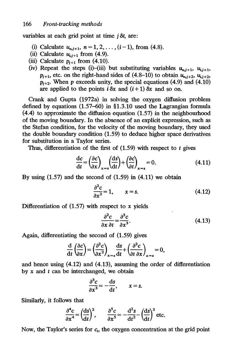
166
Front-tracking methods
variables at each grid point at time
j
8t,
are:
(i)
Calculate
u..,i+l,
n = 1, 2,
...
,
(i
-1),
from (4.8).
(ii) Calculate Uy+1 from (4.9).
(iii) Calculate
Pi+1 from (4.10).
(iv)
Repeat
the
steps (i)-(iii) but substituting variables Un.j+l> U;,j+l>
pj+h
etc. on the right-hand sides of (4.8-10) to obtain Un.j+2, Uj,i+2,
Pj+2' When P exceeds unity, the special equations (4.9) and (4.10)
are applied
to
the
points i
8x
and
(i
+ 1) 8x and so on.
Crank and
Gupta
(1972a) in solving the oxygen diffusion problem
defined by equations (1.57-60) in §1.3.10 used
the
Lagrangian formula
(4.4) to approximate
the
diffusion equation (1.57) in
the
neighbourhood
of the moving boundary.
In
the
absence of an explicit expression, such as
the Stefan condition, for
the
velocity of
the
moving boundary, they used
the
double boundary condition (1.59)
to
deduce higher space derivatives
for substitution in a Taylor series.
Thus, differentiation of
the
first of (1.59) with respect
to
t gives
dc=(ac)
(dS) +
(ac)
=0
(4.11)
dt
ax
x=s
dt
at
x=s
•
By using (1.57) and
the
second of (1.59) in (4.11) we obtain
x=S.
Differentiation of (1.57) with respect to x yields
a
2
c a
3
c
ax
at
=
ax
3
'
Again, differentiating the second of (1.59) gives
~
r
ac
) =
(~C)
ds
+(~)
=0
dt
\ax
ax
2
X=s
dt
at
ax
x=s
'
(4.12)
(4.13)
and hence using (4.12) and (4.13), assuming
the
order of differentiation
by
x and t can
be
interchanged, we obtain
Similarly, it follows that
a
4
c =
(dS)2
ax4
dt'
x=S.
aSc
= _ d
2
s _ (dS)3 etc.
ax
s
dt
2
dt
Now, the Taylor's series for G,
the
oxygen concentration at
the
grid point
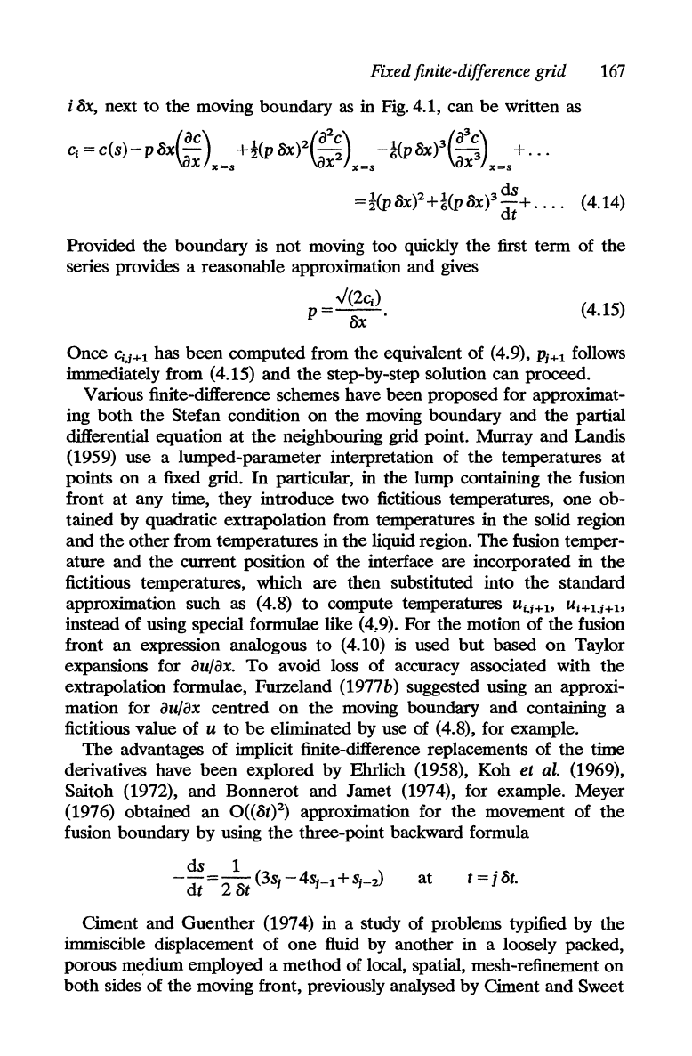
Fixed finite-difference grid
167
i 8x, next
to
the
moving boundary
as
in Fig. 4.1, can
be
written as
C
i
=C(S)-P8X(ac)
+t(p8x)d~2~)
_i(p8X)3(a3~\
+
...
ax
x=.
\ax
x=.
ax
"x=.
1(P
)2
l(
3 ds
=2
8x +6
p8x)
dt
+
....
(4.14)
Provided the boundary is not moving too quickly
the
first term of the
series provides a reasonable approximation and gives
../(2<:;)
p=~.
(4.15)
Once
c;'i+l
has been computed from the equivalent of (4.9),
Pi+1
follows
immediately from
(4.15) and
the
step-by-step solution can proceed.
Various finite-difference schemes have been proposed for approximat-
ing both
the
Stefan condition
on
the moving boundary and the partial
differential equation at the neighbouring grid point. Murray and Landis
(1959) use a lumped-parameter interpretation of
the
temperatures at
points on a fixed grid.
In
particular, in the lump containing
the
fusion
front
at
any time, they introduce two fictitious temperatures, one ob-
tained by quadratic extrapolation from temperatures in
the
solid region
and
the
other from temperatures in the liquid region.
The
fusion temper-
ature and the current position of the interface are incorporated in the
fictitious temperatures, which are then substituted into
the
standard
approximation such as
(4.8)
to
compute temperatures
Ui.i+b
Ui+1.i+b
instead of using special formulae like (4,9). For the motion of the fusion
front an expression analogous
to
(4.10)
is
used
but
based
on
Taylor
expansions for
au/ax.
To
avoid loss of accuracy associated with the
extrapolation formulae, Furzeland
(1977b) suggested using an approxi-
mation for
au/ax centred on the moving boundary and containing a
fictitious value of
u
to
be
eliminated by use of (4.8), for example.
The
advantages of implicit finite-difference replacements of the time
derivatives have been explored by Ehrlich
(1958), Koh et al. (1969),
Saitoh (1972), and Bonnerot and Jamet (1974), for example. Meyer
(1976) obtained an O«8t)2) approximation for
the
movement of
the
fusion boundary by using
the
three-point backward formula
ds
1
-
dt
= 2 8t
(3Sj
- 4Sj-l +
Sj-~
at
t=j8t.
Ciment and Guenther (1974) in a study of problems typified by
the
immiscible displacement of one fluid by another in a loosely packed,
porous medium employed a method of local, spatial, mesh-refinement on
both sides of the moving front, previously analysed by Ciment and Sweet
168
Front-tracking methods
(1973). They also incorporated the idea used earlier by Douglas and
Gallie (1955), described in §4.3.1, of adjusting the time step so
that
the
moving boundary coincided with
one
of the refined mesh points.
Huber
(1939) used
an
implicit scheme for approximating the heat-flow
equation in each time step,
but
he
tracked the moving boundary explicitly
using the Stefan condition. Rubinstein (1971) simplified
Huber's
numeri-
cal scheme and Fasano and Primicerio (1973) proved convergence
of
order
!.
In
a monumental work, Lazaridis (1970) used explicit finite-difference
approximations
on
a fixed grid
to
solve two-phase solidification problems
in both two and three space dimensions.
He
wrote
the
heat-balance
condition
on
the solidification boundary in Patel's form (see
eqn
(1.56),
§ 1.3.9) and developed numerical schemes based
on
an
a~iary
set of
differential equations which express the fact that the moving boundary
is
an isotherm. These auxiliary forms are compatible with Patel's expression
(1.56) in enabling
the
boundary movement
to
be
computed in
the
directions of
the
coordinate axes rather than along the normals to itself.
Standard finite-difference approximations to
the
heat
flow
equation were
used
at
grid points far enough from the solidification boundary.
Near
the
boundary, formulae for unequal intervals such as (4.5) and (4.7) were
incorporated into the auxiliary equations.
To
avoid loss of accuracy
associated with singularities which can arise when the moving boundary
is
too near a grid point, localized quadratic temperature profiles were used.
The manipulation
is
very complicated indeed.
In
fact, Lazaridis (1970)
merely outlined
the
derivation of his equations for the two-dimensional
case only and referred
to
his thesis (1969) for details
and
for
the
development of the three-dimensional relationships. Results were
pre-
sented for solidification problems in a prism of square cross-section and
for a three-dimensional corner.
4.3. Modified
grids
Various ways
of
modifying
the
grid have been proposed, all with the
aim of avoiding the increased complication and loss of accuracy as-
sociated with unequal space intervals near the moving boundary.
4.3.1. Variable time step
Douglas and Gallie (1955) rather than using a fixed time step and
searching for the boundary decided to determine, as
part
of
the
solution,
a variable time step such that the moving boundary coincides with a grid
line in space
at
each time level. They treated the problem defined by
the
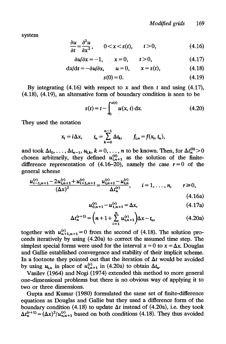
Modified grids
169
system
O<x<s(t),
t>O,
au/ax
=-1,
x=O,
t>O,
dx/dt
= -au/ax, u = 0, x = s(t),
s(O)
=0.
(4.16)
(4.17)
(4.18)
(4.19)
By integrating (4.16) with respect
to
x and then t and using (4.17),
(4.18), (4.19),
an
alternative form of boundary condition
is
seen
to
be
["<t)
s(t) =
t-
.10
u(x, t) dx.
(4.20)
They used the notation
t.n =
f(~,
t,.),
and took
at
o
,
...
,
at,.-I,
Uj,k, k = 0,
...
, n
to
be
known. Then, for
at~O)
> 0
chosen arbitrarily, they defined
U~~+1
as the solution of the finite-
difference representation of (4.16-20), namely the case
r=O
of the
general scheme
<r) 2
(r)
+
<r)
Ut-l.n+l -
UI.n+l
Ui+l.n+l
i =
1,
...
, n,
(ax)2
u8:~+1
-
ut?n+1
=
ax,
at<r+l) =
(n+1+
f
u~r)
)AX-t
n
~
~+1U
~
1=1
r;;;;OO,
(4. 16a)
(4. 17a)
(4.20a)
together with
u~tl.n+1
=0
from the second of (4.18).
The
solution pro-
ceeds iteratively by using (4.20a) to correct the assumed time step.
The
simplest special forms were used for the interval x = 0
to
x =
ax.
Douglas
and Gallie established convergence and stability of their implicit scheme.
In a footnote they pointed
out
that
the
iteration of
at
would
be
avoided
by using
Uj.n
in place
of
U~~~+1
in (4.20a)
to
obtain at,..
Vasilev (1964) and Nogi (1974) extended this method to more general
one-dimensional problems
but
there
is
no obvious way of applying
it
to
two
or
three
dimensions.
Gupta
and Kumar (1980) formulated the same set of finite-difference
equations as Douglas and Gallie but they used a difference form of
the
boundary condition (4.18)
to
update
at
instead
of
(4.20a), i.e. they took
at~+1)=(ax)2/u~~+1
based
on
both conditions (4.18). They thus avoided
170
Front-tracking methods
the
instability which develops as x increases and (4.20a) enters a closed
loop because it becomes very sensitive
to
rounding errors. Goodling and
Khader (1974) incorporated their finite-difference form of (4.18) into
the
system of equations
to
be
solved for an arbitrary value of
u~!n+1
which
is
then updated by (4. 17a). Gupta and Kumar (1981a) in a study of a
convective boundary condition
at
the
fixed end found this latter method
fails
to
converge as x increases because it
is
too sensitive
to
a small
change in
u",n+1'
Gupta and Kumar's (1981a) results are in good agree-
ment with those obtained by the other variable time-step methods and by
a Goodman's (1958) integral method (see §3.5.4).
Yuen and Kleinman (1980) used another way of updating
at
by
successive approximation.
Gupta and Kumar
(1981b) adapted the method of Douglas and Gallie
(1955)
to
solve
the
oxygen diffusion problem (see §1.3.10).
Other
authors
have
to
introduce interpolation
or
extrapolation procedures for calculat-
ing the total absorption time at which the moving boundary, marking
the
innermost penetration of oxygen, reaches
the
outer fixed surface.
In
Gupta and Kumar's method,
the
total absorption time emerges from
the
final step in
the
normal computing procedure. Their results for the
position of
the
moving boundary are compared with others in Table 4.1:
Hansen and Hougaard (1974) predicted the total absorption time
to
be
between 0.1972 and 0.1977. Gupta and Kumar (1981b) obtained 0.1973
which
is
close
to
the
accurate value of 0.197434 obtained by Dahmardah
and Mayers (1983) (see §5.1).
Kumar (1982) discussed in detail various variable time-step methods
and their application
to
problems mentioned above and
to
others includ-
ing phase-change with non-uniform initial temperatures, time-dependent
boundary conditions,
the
dissolution of a spherical gas bubble in a liquid,
and the freezing of liquid inside and outside a cylinder.
For
most
problems, numerical results obtained by several methods were compared.
4.3.2. Variable
space
grid
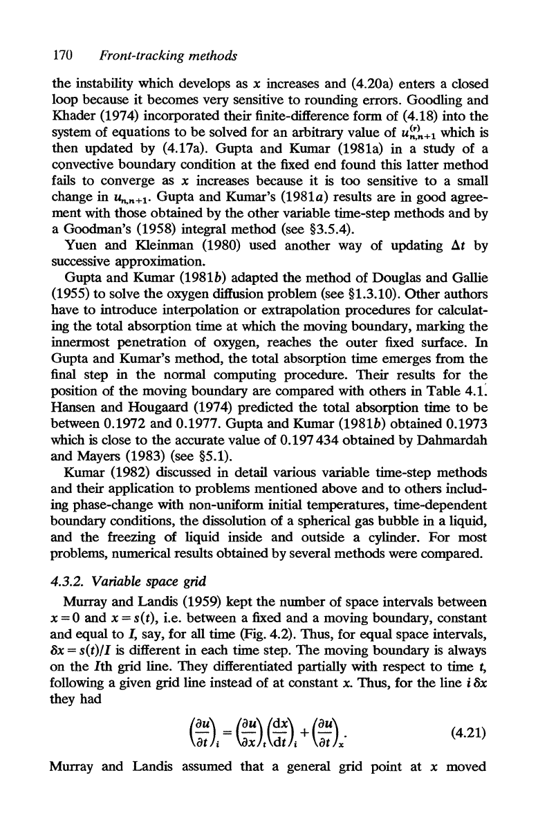
Murray and Landis (1959) kept
the
number of space intervals between
x = 0 and x = s(t), i.e. between a fixed and a moving boundary, constant
and equal
to
I,
say, for all time (Fig. 4.2). Thus, for equal space intervals,
8x =
s(t)/l
is different in each time step. The moving boundary is always
on
the
lth
grid line. They differentiated partially with respect
to
time
t,
following a given grid line instead of
at
constant
x.
Thus, for the line i 8x
they had
(4.21)
Murray and Landis assumed
that
a general grid point
at
x moved
Modified
grids
171
I
I
I
r----.r----,-----,----~I
j
!
.I
//
I~"""
~--_+----~LL---~----~~
I / I
/,1
I / /
FIG. 4.2. Murray and Landis variable grid
according
to
the
expression
dXj
Xj
ds
dt"=
S(t)
dt·
The
one-dimensional heat equation becomes
(
au\
x ds
au
ifu
atJi
=
s(t)
dt
ax
+
ax
2
'
x
(4.22)
(4.23)
and
s(t)
is
updated
at
each time step by using, for example, a suitable
finite-difference form of
the
boundary condition ds/dt =
-au/ax
on
x =
s(t).
The
method was extended by Heitz and Westwater (1970) to
convection problems and by Tien and Churchill (1965) to cylindrical
geometry.
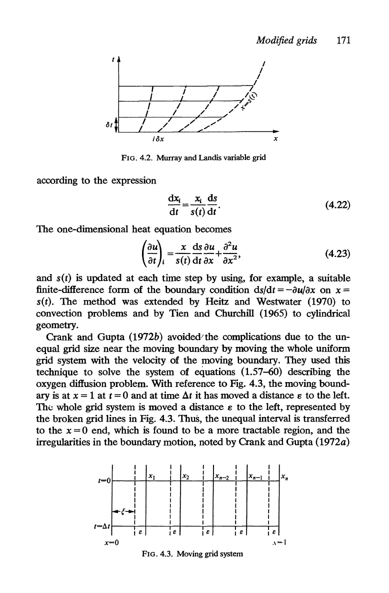
Crank and Gupta
(1972b) avoidedtthe complications due
to
the un-
equal grid size near the moving boundary by moving the whole uniform
grid system with
the
velocity of
the
moving boundary. They used this
technique
to
solve the system of equations (1.57-60) describing the
oxygen diffusion problem. With reference
to
Fig. 4.3,
the
moving bound-
ary
is
at
x = 1
at
t = 0 and
at
time
at
it has moved a distance E
to
the
left.
The whole grid system is moved a distance
E to
the
left, represented
by
the
broken grid lines in Fig. 4.3. ThuS,
the
unequal interval
is
transferred
to
the x = 0 end, which
is
found to
be
a more tractable region, and the
irregularities in the boundary motion, noted by Crank and Gupta
(1972a)
I
I I
I
I
1-0
I
:
I
I I
I
XI
X2
I
X
n
-2
I
Xn-I
I
: :
I
I
I
I
I
I
I
I
I
I
I I I
I I
I
I
I I I
r--(--:
I
I
I I
I I
I
I
I I I
I I
Ie
Ie
Ie
I e
Ie
X-o
.,-1
FIG. 4.3. Moving grid system