Crank J. Free and Moving Boundary Problems
Подождите немного. Документ загружается.

172
Front-tracking methods
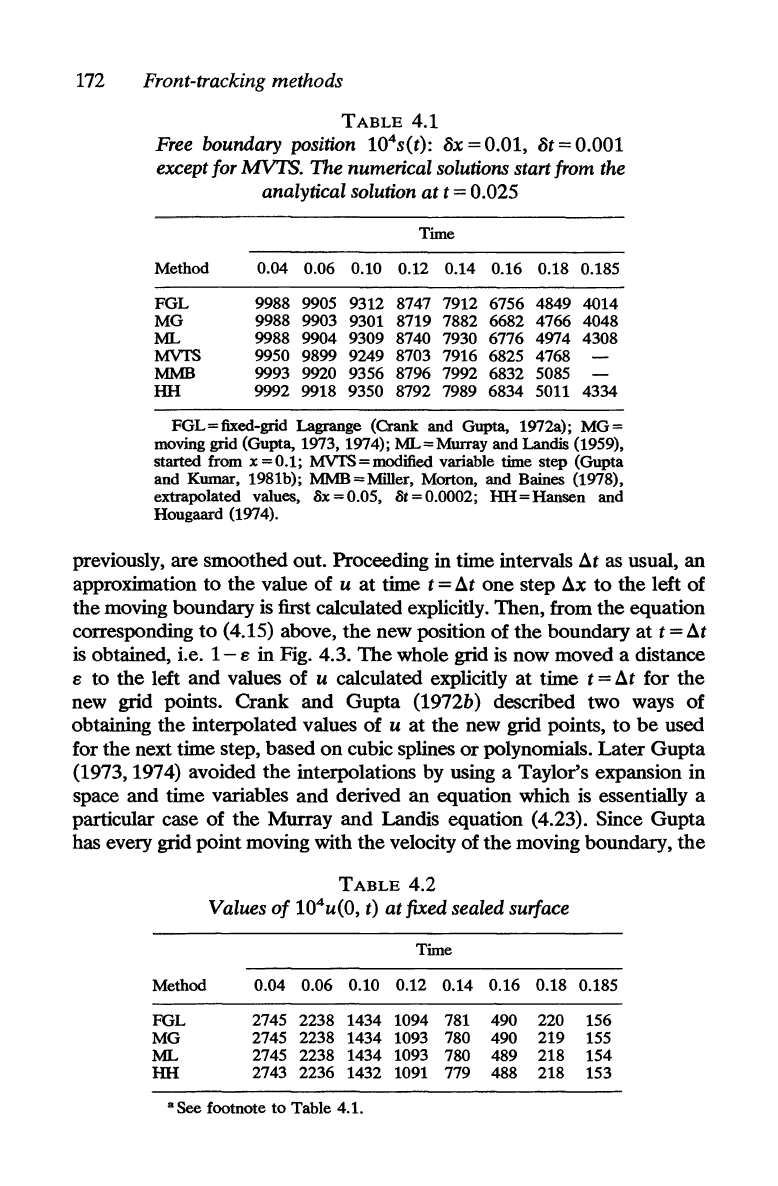
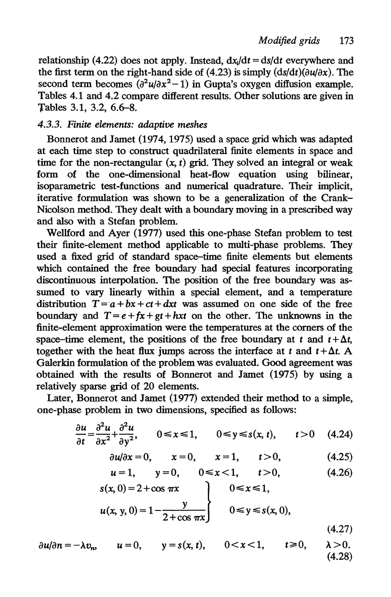
TABLE
4.1
Free boundary position 104s(t): 8x = 0.01, 8t = 0.001
except for MVTS. The numerical solutions start from the
analytical solution
at
t = 0.025
Time
Method 0.04
0.06
0.10 0.12 0.14
0.16 0.18 0.185
FGL
9988 9905
9312
8747 7912
6756 4849 4014
MG
9988 9903
9301
8719 7882 6682 4766 4048
ML
9988 9904 9309 8740 7930 6776 4974 4308
MVI'S
9950 9899
9249
8703 7916 6825 4768
MMB
9993 9920 9356 8796 7992 6832 5085
-
HH
9992
9918 9350 8792 7989 6834 5011 4334
FGL=fixed-grid
Lagrange (Crank and Gupta, 1972a);
MG=
moving grid (Gupta, 1973, 1974);
ML=Murray
and Landis (1959),
started
from x
=0.1;
MVI'S=modified variable time step (Gupta
and Kumar, 1981b);
MMB=Miller,
Morton,
and
Baines (1978),
extrapolated values,
8x = 0.05, at = 0.0002;
HH
= Hansen and
Hougaard (1974).
previously, are smoothed out. Proceeding in time intervals
at
as usual,
an
approximation
to
the
value
of
u
at
time t =
at
one
step
ax
to
the
left
of
the
moving boundary is first calculated explicitly. Then, from
the
equation
corresponding
to
(4.15) above,
the
new position
of
the
boundary
at
t
=at
is
obtained, i.e.
1-
8 in Fig. 4.3.
The
whole grid is now moved a distance
8
to
the
left
and
values
of
u calculated explicitly
at
time t =
at
for
the
new grid points. Crank and
Gupta
(1972b) described two ways
of
obtaining
the
interpolated values
of
u
at
the
new grid points,
to
be
used
for
the
next time step, based
on
cubic splines
or
polynomials.
Later
Gupta
(1973,1974) avoided
the
interpolations by using a Taylor's expansion in
space and time variables
and
derived
an
equation which is essentially a
particular case
of
the
Murray
and
Landis equation (4.23). Since
Gupta
has every grid point moving with
the
velocity
of
the
moving boundary,
the
TABLE
4.2
Values
of
10
4
u(0, t)
at
fixed sealed surface
Time
Method 0.04
0.06
0.10 0.12
0.14
0.16 0.18
0.185
FGL
2745
2238 1434 1094 781 490
220
156
MG
2745 2238 1434 1093 780
490
219
155
ML
2745
2238 1434
1093
780 489
218
154
HH
2743 2236 1432 1091 779 488
218
153
-See
footnote
to
Table 4.1.
Modified grids
173
relationship (4.22) does
not
apply. Instead, dxddt = ds/dt everywhere and
the first term
on
the right-hand side of (4.23)
is
simply (ds/dt)(au/ax). The
second term becomes
(a
2
u/ax2-1)
in Gupta's oxygen diffusion example.
Tables 4.1 and 4.2 compare different results. Other solutions are given in
Tables 3.1, 3.2, 6.6-8.
4.3.3. Finite elements: adaptive meshes
Bonnerot and Jamet (1974, 1975) used a space grid which was adapted
at
each time step
to
construct quadrilateral finite elements in space and
time for the non-rectangular
(x,
t)
grid. They solved an integral or weak
form of the one-dimensional heat-flow equation using bilinear,
isoparametric test-functions and numerical quadrature. Their implicit,
iterative formulation was shown to be a generalization of the
Crank-
Nicolson method. They dealt with a boundary moving in a prescribed way
and also with a Stefan problem.
Wellford and Ayer (1977) used this one-phase Stefan problem to test
their finite-element method applicable
to
multi-phase problems. They
used a fixed grid of standard space-time finite elements but elements
which contained the free boundary had special features incorporating
discontinuous interpolation. The position of the free boundary
was as-
sumed
to
vary linearly within a special element, and a temperature
distribution
T
=a
+ bx + ct +
dxt
was assumed
on
one side of the free
boundary and
T = e +
fx
+ gt +
hxt
on the other. The unknowns in the
finite-element approximation were the temperatures at
the
corners of
the
space-time element,
the
positions of the free boundary
at
t and t +
at,
together with
the
heat flux jumps across the interface
at
t and t +
at.
A
Galerkin formulation of the problem
was evaluated. Good agreement was
obtained with the results of Bonnerot and Jamet (1975) by using a
relatively sparse grid of 20 elements.
Later, Bonnerot and Jamet (1977) extended their method
to
a simple,
one-phase problem in two dimensions, specified as follows:
0.:;;x.:;;1, O.:;;y .:;;s(x, t),
au/ax
=0,
x
=0,
x = 1,
t>O,
u=1,
y=O,
0':;;x<1,
t>O,
t>O
(4.24)
(4.25)
(4.26)
s(x,
0)
= 2 + cos
1TX
y } 0':;;x':;;1,
u(x,
y,
0)
= 1
2+
cos
1TX
O.:;;y .:;;s(x, 0),
u=O,
y = s(x, t),
0<x<1,
t;;;:.O,
(4.27)
.\.>0.
(4.28)
174
Front-tracking methods
4.01------.
4.0
I
\
(b)
y
/
\
/
x
o
x
1.0
p.+!
I
(c)
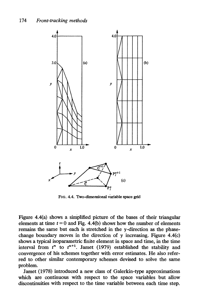
FIG. 4.4. Two-dimensional vanable space grid
Figure 4.4(a) shows a sinlplified picture of the bases of their triangular
elements at time
t = 0 and Fig. 4.4(b) shows how the number of elements
remains
the
same
but
each
is
stretched in
the
y-direction as the phase-
change boundary moves in
the
direction of y increasing. Figure 4.4(c)
shows a typical isoparametric finite element in space and time, in the time
interval from
t
n
to
tn+l.
Jamet (1979) established the stability and
convergence of his schemes together with error estimates.
He
also refer-
red
to
other similar contemporary schemes devised
to
solve
the
same
problem.
Jamet (1978) introduced a new class of Galerkin-type approximations
which are continuous with respect
to
the space variables
but
allow
discontinuities with respect
to
the time variable between each time step.
Modified grids
175
Thus
the
elements may
be
chosen arbitrarily at each time step with no
connection with the elements corresponding to the previous step. This
is
a
more flexible procedure than the one mentioned above (Bonnerot and
Jamet 1974, 1975),
but
the general mathematical theory was developed
only for a prescribed moving boundary and no numerical experiments
were reported. Subsequently, Bonnerot and Jamet (1979) proposed a
third-order-accurate discontinuous finite-element method for a one-
dimensional Stefan problem, based
on
biquadratic finite elements. This
work
will now
be
described in more detail.
Bonnerot and Jamet (1979) solve the following problem:
au
;Pu
iit=
dX
2
'
u(x, 0) =
UO(x),
0
<:;;x
<:;;
aO,
u(O,t)=g(t),
O<t~T,
u(a(t),
t) = 0,
O<t~T,
da
dU
-=-c-
dt
dX'
x =
a(t),
a (0) =
aO,
(4.29)
(4.30)
(4.31)
(4.32)
(4.33)
(4.34)
where
a(t)
is
an unknown, positive function specifying the position of the
Stefan phase-change boundary which starts
at
a(O) =
aO.
The partial
differential equation
is
replaced by
t~e
integral relation
I
tn
+1
1a(t)
de(>
I
tn
+'l
a(t)
dU
de(>
- u - dx
dt
+ -
-::r
dx
dt
n dt n °
dX
oX
r a
(t
n
+ 1) r
a(t
n
)
+ k u(X, t
n
+
1
)e(>(x,
t
n
+
1
)
dx - k u(X,
tn)e(>(x,
t
n
)
dx
= 0, (4.35)
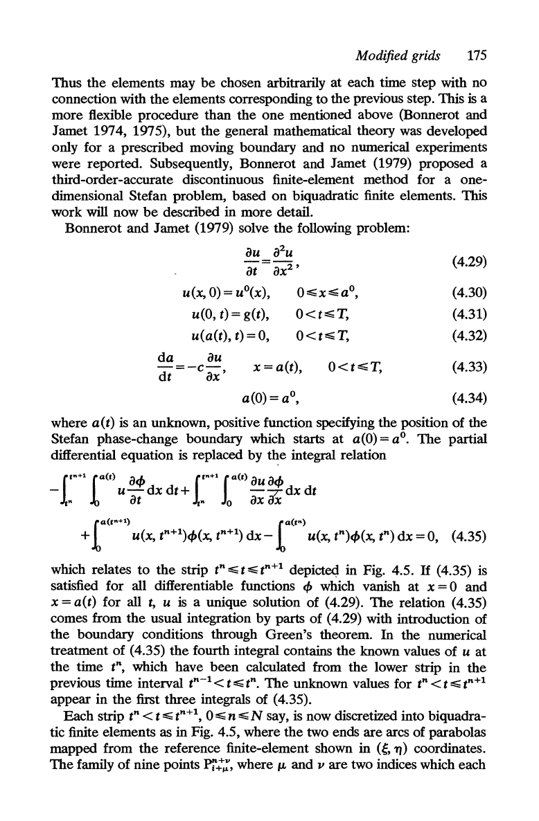
which relates
to
the
strip t
n
<:;;t<:;;t
n
+1
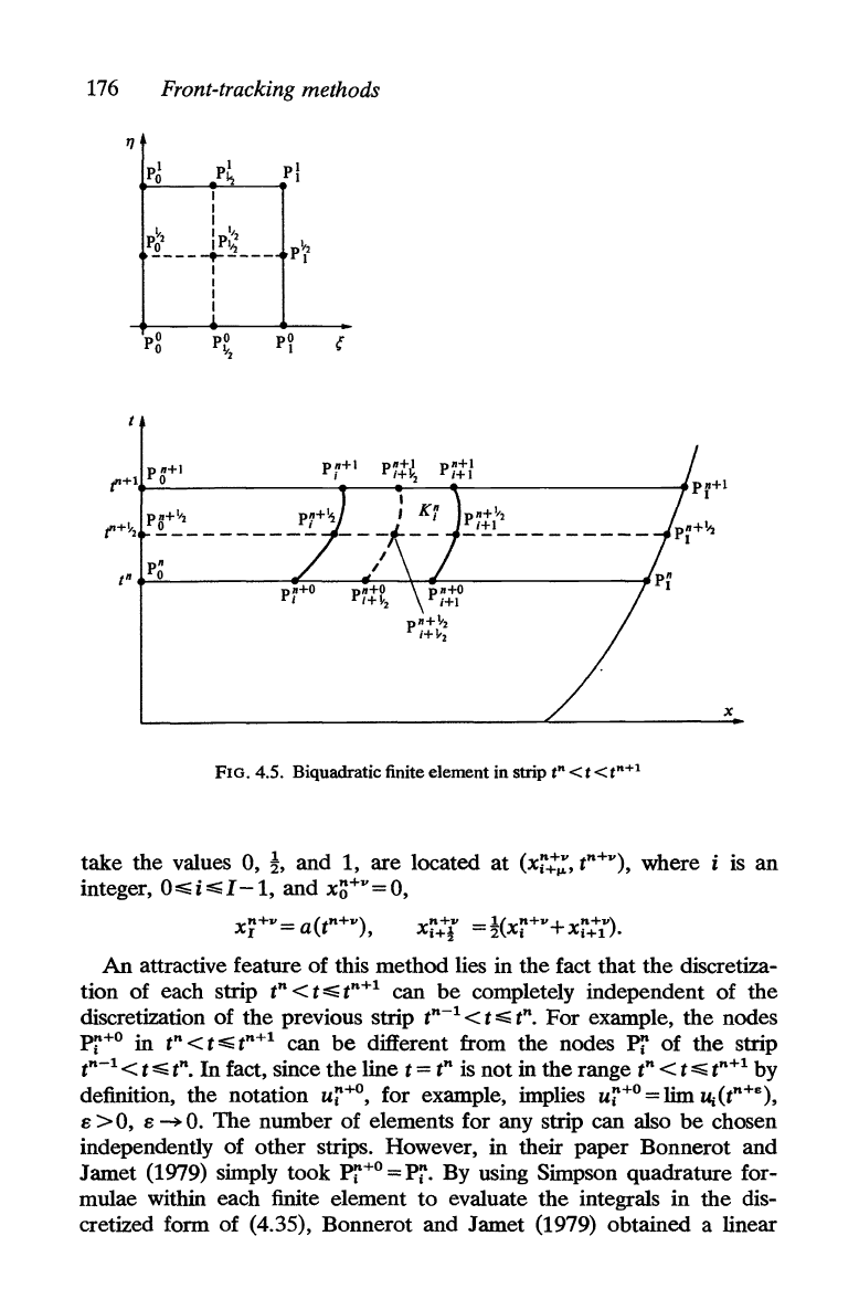
depicted in Fig. 4.5.
If
(4.35)
is
satisfied for all differentiable functions
e(>
which vanish
at
X = 0 and
x = a(t) for all
t,
u
is
a unique solution of (4.29). The relation (4.35)
comes from
the
usual integration by parts of (4.29) with introduction of
the boundary conditions through Green's theorem. In the numerical
treatment of (4.35)
the
fourth integral contains
the
known values of u
at
the time
tn,
which have been calculated from the lower strip in the
previous time interval
t
n
-
1
<t<:;;t
n
•
The
unknown values for t
n
<t<:;;t
n
+
1
appear in
the
first three integrals of (4.35).
Each strip
t
n
< t
<:;;
tn+t, 0
<:;;
n
<:;;N
say,
is
now discretized into biquadra-
tic finite elements as in Fig. 4.5, where the two ends are arcs of parabolas
mapped from
the
reference finite-element shown in
(e,
'l))
coordinates.
The
family of nine points Pi::, where
JL
and v are two indices which each
176
Front-tracking methods
TJ
pn+l
('+1
0
pO
l-,
pO
1
p~+1
I
pn+l.ll
('+~2
~
________
_
FIG. 4.5. Biquadratic finite element in strip
t"<t<t"+l
x
take
the values 0,
!,
and 1, are located
at
(xr.:;,
t
n
+,,),
where
is
an
integer,
0,..;i,..;I-1,
and
x~+"=O,
An
attractive feature
of
this method lies in
the
fact
that
the
discretiza-
tion
of
each strip
tn<t,..;t
n
+
1
can
be
completely independent
of
the
discretization
of
the previous strip t
n
-
1
<
t,..;
tn.
For
example,
the
nodes
pr+
o
in t
n
<
t"';
t
n
+
1
can
be
different from the nodes
~
of
the
strip
t
n
-
1
< t"';
tn.
In
fact, since
the
line t = t
n
is
not in
the
range t
n
<
t.:;;;
t
n
+
1
by
definition, the notation
ur+
o
,
for example, implies
ur+
o
=
lim
U;(t
n
+,,),
E > 0, E
~
O.
The
number of elements for any strip can also
be
chosen
independently
of
other
strips. However, in their
paper
Bonnerot and
Jamet (1979) simply took
~+o
=
pro
By using Simpson quadrature for-
mulae within each finite element
to
evaluate
the
integrals in the dis-
cretized
fonn
of
(4.35), Bonnerot and Jamet (1979) obtained a linear
Modified grids
177
system of equations with a square matrix. They give details for computing
the
coefficients.
In
order
to
gain
one
order of accuracy, Bonnerot and Jamet (1979)
approximated the derivative
au/ax =
Du(t),
say,
in
the
moving boundary
condition (4.33), as follows. Denote by
v~+v
the function of x obtained by
cubic interpolation of the values
ui:: at the nodes
Pi::
for i +
f.J.
= I
-~,
I
-1,
I
-!,
and
I.
Let
(Du)~+v
denote avn+v/ax
at
the end-point Pj+v and
approximate
Du(t)
in
the
interval t
n
<t..;;t
n
+1
by the function (DU)h(t)
obtained by quadratic interpolation of the three values of
(Du)~+v
for
v = O,!, 1.
The
moving boundary condition (4.33) can now
be
discretized.
The curve
x = a(t) is approximated by a continuous curve x =
ah
(t) which
in
each interval
tn..;;
t:os;
t
n
+
1
is a section of a parabola x =
q~n)(t),
which
denotes a polynomial of degree
..;;2
with respect
to
the
variable
t.
Let
a
n
+
v
= ah(t
n
+
v
).
At
each time step,
the
values of a
n
+!
and a
n
+1
are
computed from the integrated form of (4.33) with respect
to
t;
a
n
+
v
= an - c
Ift+.
(DU)h(t)
dt
(4.36)
for
v=!
and 1, where (DU)h(t) denotes the approximation of
Du(t)
obtained by quadratic interpolation above.
An
iterative procedure
is
now needed since the values of (DU)h(t) in
the
interval t
n
<
t..;;
t
n
+
1
depend
on
the computed values of
Uh
in this strip
which in
turn
depend
on
a
n
+
t
and a
n
+
1
•
Bonnerot and Jamet (1979)
adopted the following iterative procedure:
(i)
Given values
at
the t'th stage of the iteration denoted by
an+!.e,
a
n
+
1
.
e
,
Uh(X,
t)e, calculate {(DU)h(tW as above;
(ii) Calculate a
n
+!.e+1
a
n
+
1
,e+1
by inserting {(DU)h(tW in (4.36).
The
iterations are started from.
an+v,o
=
q~-l(tn+v)
for v =! and 1, n
;.01,
i.e. from the quadratic extrapolation of
an-I,
a
n
-!, and an. For n = 0,
a
1.0
=
a!'O
=
aO
is
used.
Bonnerot and Jamet (1979) claimed that their method has the further
advantage that it
is
specially well suited
to
handle problems with sin-
gularities, e.g. discontinuities in the initial functions
UO(x),
or
in the
boundary values including an initial discontinuity
on
the free boundary
which then moves with infinite speed at
t = 0. They quoted numerical
results
to
establish that the convergence
is
of order 3 even in computing a
discontinuity, and
that
their method
is
unconditionally stable. They also
demonstrated that initial singularities generate
no
irregularity of the
computed values
at
later times, such as the oscillations which are often
178
Front-tracking methods
produced by
other
methods, and
that
the accuracy remains very satisfac-
tory.
Bonnerot and Jamet (1981) applied a modified and extended form of
their third-order-accurate discontinuous finite-element method
to
solve
the
one-dimensional Stefan problem involving three phases which appear
and disappear described in §1.3.6. Their scheme is conservative.
One
interesting feature of their results
is
that
when they appear the moving
boundaries start with zero initial speed.
For
mathematical results con-
cerning appearing and disappearing phases
the
reader
is
referred
to
Cannon and Primicerio (1973); Cannon et
at.
(1967); and Sherman
(1971).
Miller, Morton, and Baines (1978) described a method which is closely
similar
to
that
of Bonnerot and Jamet (1974, 1975)
but
they used finite
differences in time with finite elements in space which are of standard
length apart from the last two, which are adapted
at
each time step
to
fit
the new position
of
the
moving boundary. Miller et
al.
(1978) studied
the
oxygen diffusion problem defined by equations (1.57-60).
They represented
the
approximate solution
at
the
discrete times
t,.,
n =
,1,
2,
...
, as
J
Un(x)
= L
Ojq,j(x),
(4.37)
j=l
The
coefficients
OJ
are
to
be
calculated so as
to
give
the
best representa-
tion of
u(x,
t,.)
in
eqn
(1.57) in terms
of
the basis functions q,j(x), in
the
least-squares sense.
An
appropriate weak form
of
the
differential equa-
tion
is
obtained in
the
usual way by multiplying (1.57)
by
a suitable test
function
I/I(x), integrating over x and t, and using
the
boundary conditions
(1.58) and (1.59).
The
weak form is
J.
xo(tft+1)
rXo(t
ft
)
o u(x, t,.+l)I/I(X) dx - k u(x, t,.)I/I(x) dx
= -
fft+1
dt[fo(t)
I/Ixttx
dx +
fo(t)
I/I(x) dx
].
(4.38)
When
u
is
replaced by U and
1/1
by
q,r+1,
and
the
6-method quadrature is
applied
to
the
right-hand side of (4.38), the Galerkin equations which
determine
the
OJ
in (4.37) are
J
[J.
XO(tft+l)
dU"+l
d.l.
n
+
1
{U"+1(x)-un(x)}q,r+1(x)dx
=-6ilt
___
'I'_i_dx
o dx
dx
Substitution
of
(4.37) into
the
approximated form
of
(4.38) produces
the
Modified grids
179
system
of
equations
[M+
6(t,.+1- t,.)K]Qn+1 =
R-(t,.+1-
t,.)S,
(4.39)
where
and
M
and
K
are
the
usual mass
and
stiffness matrices
at
time level t..+l
given by
Linear basis functions
are
used throughout.
In
the
interests
of
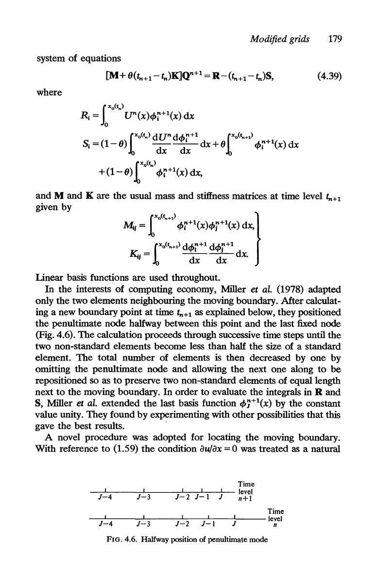
computing economy, Miller
et
al. (1978) adapted
only
the
two elements neighbouring
the
moving boundary.
After
calculat-
ing a new boundary
point
at
time t..+l as explained below, they positioned
the
penultimate
node
halfway between this point
and
the
last fixed node
(Fig. 4.6).
The
calculation proceeds through successive time steps until
the
two non-standard elements become less
than
half
the
size
of
a standard
element.
The
total
number
of
elements is
then
decreased by
one
by
omitting
the
penultimate node
and
allowing
the
next
one
along
to
be
repositioned so as
to
preserve two non-standard elements
of
equal length
next
to
the
moving boundary.
In
order
to
evaluate
the
integrals in
Rand
S, Miller et al. extended
the
last basis function
cfr
1
(x) by
the
constant
value unity. They found by experimenting with
other
possibilities
that
this
gave
the
best results. -
A nove] procedure was adopted for locating
the
moving boundary.
With reference
to
(1.59)
the
condition
au/ax
= 0 was treated as a natural
Time
I I I I I
level
J-4
J-3
J-2
J-l
J
n+l
Time
I
I
I
I I
level
J-4
J-3
J-2
J-l
J
"
FIG. 4.6. Halfway position of penultimate mode
180
Front-tracking methods
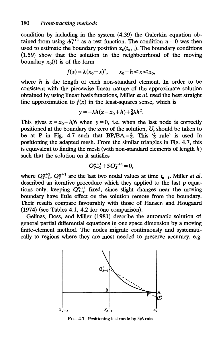
condition by including in the system (4.39) the Galerkin equation ob-
tained from using
</>;+1
as
a test function.
The
condition u = 0 was then
used to estimate
the
boundary position
XO(tn+1)'
The
boundary conditions
(1.59) show that the solution in the neighbourhood of the moving
boundary
xo(t)
is
of
the
form
{(x)=A(xo-xf,
xo-h~x~xo,
where h
is
the
length of each non-standard element.
In
order
to
be
consistent with the piecewise linear nature of
the
approximate solution
obtained by using linear basis functions, Miller
et
al.
used
the
best straight
line approximation
to
f(x)
in
the
least-squares sense, which
is
y
=-Ah(x-xo+h)+iAh
2
•
This gives x = Xo - h/6 when y = 0, i.e. when the last node
is
correctly
positioned at the boundary
the
zero of the solution,
U,
should
be
taken
to
be
at P
in
Fig. 4.7 such that BP/BA=i. This
'i
rule'
is
used in
positioning
the
adapted mesh. From
the
similar triangles in Fig. 4.7, this
is
equivalent
to
finding the mesh (with non-standard elements of length h)
such that the solution on it satisfies
0;~t+50;+1
=0,
where
O;~t,
0;+1 are the last two nodal values
at
time
t..+1'
Miller et
al.
described an iterative procedure which they applied
to
the
last p equa-
tions only, keeping
0;=;
fixed, since slight changes near
the
moving
boundary have little effect
on
the
solution remote from
the
boundary.
Their results compare favourably with those of Hansen and Hougaard
(1974) (see Tables 4.1, 4.2 for
One
comparison).
Gelinas, Doss, and Miller (1981) describe
the
automatic solution of
general partial differential equations in one space dimension by a moving
finite-element method. The nodes migrate continuously and systemati-
cally
to
regions where they are most needed to preserve accuracy, e.g.
r-----------~+_--------~~A
p
...
Q1
X
J
-
2
FIG. 4.7. Positioning last mode
by
5/6 rule
Method
of
lines
181
regions of high gradients. Extension
to
two dimensions
is
mentioned.
Adaptable, non-uniform grids
are
used by Jones and Thompson (1980)
to
obtain accuracy
in
finite-difference calculations.
4.4. Method
of
lines
For
problems in
one
space dimension,
the
time variable is discretized in
this method which is a well-known
one
for solving fixed-boundary prob-
lems.
The
partial differential equation
is
replaced by a sequence of
ordinary differential equations
at
discrete time levels. Meyer
(1970, 1977a,b,c, 1978a,b,c) developed
the
method in relation
to
moving
boundary problems in a consistent
and
generalized way.
The
1977c
paper
contains references
to
earlier solutions
of
sundry isolated problems by
various authors.
We
introduce
the
method
of lines through
the
one-dimensional two-
phase Stefan problem specified
by
~
(k
aUt)
_ c aUt = F
ax
t
ax
t
at
I>
b
t
<x<s(t),
t>O
(4.41)
~(k
aU2)_C
aU2=F
ax
2
ax
2
at
2,
s(t)<x<b
2
,
t>o,
(4.42)
aUt
x =bl>
t>o,
(4.43)
U
t
=
I3t(t)-+at(t),
ax
aU2
x=b
2
,
t>o,
(4.44)
-=
132(t)u2+
a2
t
,
ax
where
kl>
Ch
FI> k2'
C2,
F2
may
be
functions
of
x and
t,
e.g. k
t
=
kt(x,
t),
etc.
On
the
free boundary
s(t)
we
have
the
conditions
U2
= ILz(S(t), t),
aUt
aU2
ds
k
t
--
k2
-+
A(S(t), t)
-d
= 1L3(S(t), t),
ax
ax
t
x
=
s(t),
(4.45)
t>o,
(4.46)
Meyer
(1978b) showed
that
the
introduction of convection terms
aUt/ax,
aU2/aX
causes
no
further difficulty.