Dantzig G., Thapa M. Linear programming. Vol.1. Introduction

222 TRANSPORTATION AND ASSIGNMENT PROBLEM

c

11

c

12

c

13

c

14

c

15

c

21

c

22

c

23

c

24

c

25

c

21

c

22

c

23

c

24

c

25

a

1

a

2

a

3

b

1

b

2

b

3

b

4

b

5

.

x

11

.

x

21

.

x

22

.

x

32

.

x

33

.

x

34

.

x

35

u

1

u

2

u

3

v

1

v

2

v

3

v

4

v

5

θ

∗

......................................................................................................................................................................................................................................................................................................

.

−θ

.

..

.

+θ

........................................................................

.

−θ

.

..

.

+θ

..........................................................................................................................................................................................................

.

−θ

.

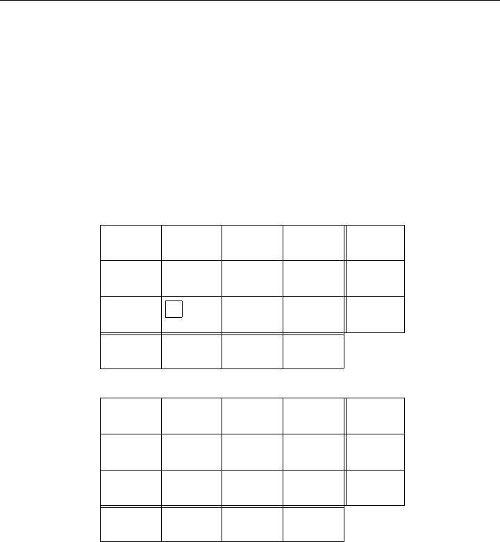
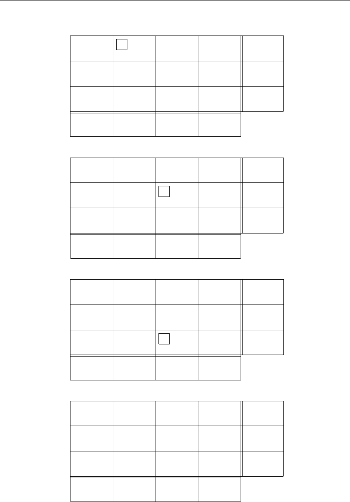
Figure 8-12: Theta-Adjustments for the Standard Transportation Array

8.4 FAST SIMPLEX ALGORITHM FOR THE

TRANSPORTATION PROBLEM

Even small general linear programs require a computer; whereas small transporta-

tion problems can be easily solved by hand using just a pencil and paper. At each

iteration of the Simplex Algorithm applied to the transportation problem, adjust-

ments are made to the x

ij

in the cells of the rectangular array in Figure 8-3. These

adjustments are sometimes referred to as theta-adjustments since a value θ of the

incoming variable is added and subtracted from some of the basic variables; see

the array in Figure 8-12, where the θ with a star, θ

∗

, refers to the position of the

entering variable.

The steps are the same as those of the Simplex Algorithm except that the

calculations of the reduced costs and the changes to the basic variables are simple

additions and subtractions.

8.4.1 SIMPLEX MULTIPLIERS, OPTIMALITY, AND

THE DUAL

In this section we show how we can take advantage of the structure of the classical

transportation problem to easily obtain the simplex multipliers and reduced costs.

SIMPLEX MULTIPLIERS

To distinguish the multipliers corresponding to the rows from those of the columns

of the transportation array, let u

i

represent the multiplier for the ith row equation,

and let v

j

represent the multiplier for the jth column equation instead of using π

k

for all equations k as we have done earlier.

The values of the u

i

and v

j

are chosen so that the basic columns price out to zero.

However, there appears to be a complication because there are m + n −1 equations

that are not redundant and m + n unknowns u

i

and v

j

(including the multiplier

8.4 FAST SIMPLEX ALGORITHM FOR THE TRANSPORTATION PROBLEM 223

on the redundant equation). Recall that any equation in (8.4) may be considered

redundant and may be dropped. Dropping is the same as saying that we can assign

an arbitrary value, say zero, to the simplex multiplier on the redundant equation

and then evaluate the remaining m + n − 1 multipliers by solving the m + n − 1

equations corresponding to the m + n − 1 basic variables. If one id doing hand

computations, a good convention is to ﬁnd a row or column having the greatest

number of basic variables and to set its corresponding price to zero. In order for a

basic column (i, j) to price out to zero, we must have

c

ij

= u

i

+ v

j

for x

ij

basic, (8.12)

because column (i, j) has exactly two nonzero coeﬃcients: +1 corresponding to

equation i in the demand equations and +1 corresponding to equation j in the

supply equations, see (8.3).

As we have seen, the basis is triangular and thus we can determine such prices

by scanning the squares corresponding to basic variables until one is found for

which either the row price, u

i

, or the column price, v

j

, has already been evaluated;

subtracting either price from c

ij

determines the other price. The triangularity of

the basis guarantees that repeated scanning will result in the evaluation of all u

i

and v

j

.

For large problems this procedure for scanning the rows and columns is not

eﬃcient. More eﬃcient methods are based on the fact that a basis of the trans-

portation problem corresponds to a tree in a graph; the tree structure can be used

to determine more eﬃciently the updated prices and changes in the values of the

basic variables. Such techniques are described for general networks in Chapter 9.

REDUCED COSTS AND OPTIMALITY

To determine whether the solution is optimal, multiply the ith row equation of (8.2)

by u

i

and the jth column equation by v

j

and then subtract the resulting equations

from the objective function to obtain a modiﬁed z-equation,

m



i=1

n



j=1

¯c

ij

x

ij

= z − z

0

, (8.13)

where the ¯c

ij

, which are the reduced costs, are given by

¯c

ij

= c

ij

− (u

i

+ v

j

) for i =1,...,m, j =1,...,n, (8.14)

and

z

0

=

m



i=1

a

i

u

i

+

n



j=1

b

j

v

j

. (8.15)

The ¯c

ij

corresponding to the basic variables are all zero by (8.12). The basic feasible

solution is optimal if ¯c

ij

≥ 0 for all the nonbasic variables.

224 TRANSPORTATION AND ASSIGNMENT PROBLEM

 Exercise 8.16 Show that any one of the m + n multipliers may be given an arbitrary

value, other than 0, in determining the remaining multiplier. Speciﬁcally, show that an

arbitrary constant k can be added to all the multipliers u

i

and subtracted from all the

multipliers v

j

, (i.e., the multipliers u

i

may be replaced by (u

i

+ k) and the multipliers v

j

may be replaced by (v

j

−k)), without aﬀecting the value of ¯c

ij

and z

0

in (8.14) and (8.15).

 Exercise 8.17 Show that if the c

ij

are replaced by c

ij

− u

i

− v

j

, where u

i

and v

j

are

arbitrary, that this does not aﬀect the optimal solution x

∗

ij

but does aﬀect the value of the

objective.

DUAL OF THE TRANSPORTATION PROBLEM

It is interesting to look at the dual of the transportation problem, i.e.,

Maximize

m



i=1

a

i

u

i

+

m



j=1

b

j

v

j

= w

subject to u

i

+ v

j

≤ c

ij

for all (i, j),

(8.16)

where u

i

, v

j

are unrestricted in sign for all (i, j). The primal variable x

ij

gives rise

to the dual constraint u

i

+ v

j

≤ c

ij

. Thus the slack variable on this dual constraint

is

y

ij

= c

ij

− u

i

− v

j

,y

ij

≥ 0, (8.17)

and, by complementary slackness, either x

ij

=0ory

ij

= 0. Thus, if x

ij

is basic we

must have y

ij

=0orc

ij

= u

i

+ v

j

, as we saw in Equation (8.12).

 Exercise 8.18 Prove that any basis of the transportation problem’s dual is triangular.

 Exercise 8.19 Prove in general that the transpose of any triangular basis is triangular.

8.4.2 FINDING A BETTER BASIC SOLUTION

As we have seen earlier, in the Simplex Method for a general linear program in

standard form, if ¯c

ij

=¯c

rs

is negative, then the corresponding nonbasic variable x

rs

is suitable as a candidate for entering into the basic set, replacing a basic variable

taht, after it is dropped from the basic set, becomes just another nonbasic variable.

The usual rule for selecting a nonbasic variable to enter the basic set is to choose

the one with the most negative reduced cost ¯c

ij

, i.e., choose x

rs

to be the new basic

variable if

c

rs

− u

r

− v

s

= min

(i, j)

(c

ij

− u

i

− v

j

) < 0. (8.18)

The triangularity of the basis makes it very easy to perform the calculations

to determine which variable will leave the basis and makes it easy to update the

8.4 FAST SIMPLEX ALGORITHM FOR THE TRANSPORTATION PROBLEM 225

values of the remaining basic variables. This is especially easy to do by hand if the

calculations are done directly on the rectangular array itself.

To start, enter the symbol θ

∗

in the cell (r, s) to indicate that a value, called

θ = θ

∗

, will be given to the entering nonbasic variable x

rs

. Next, the basic entries

are adjusted so that the row sums and column sums stay unchanged. This requires

appending (+θ) to some entries, (−θ) to others, and leaving the rest unchanged.

Because the basis is triangular, it will always be possible to locate by eye where a

single basic entry is to be converted by an unknown amount +θ or −θ or remain

unchanged. Once the locations where the +θ or −θ adjustments have to be done

have been determined, θ is replaced by x

pq

, the largest numerical value that does

not make a basic entry negative. That is, at iteration t, θ takes on the value x

t

pq

of

the smallest entry to which the symbol (−θ) is appended, so that x

t

pq

− θ becomes

zero. The variable x

pq

is then dropped from the basic set. Any basic variable whose

value is equal to x

t

pq

and which is appended by −θ may be chosen to be dropped

from the basic set. The value of θ so determined is then used to recompute all

the basic entries for the new basic solution x

t+1

. This completes the iteration and

we once again recompute the multipliers and check for optimality and repeat the

process if x = x

t+1

is not optimal.

The eye scanning procedure used above is not eﬃcient for large problems. In-

stead, the tree structure associated with the basis is exploited to eﬃciently adjust

the basic variables. Such techniques are described for general networks in Chapter 9.

 Exercise 8.20 Show that it is not possible to have z →−∞.

8.4.3 ILLUSTRATION OF THE SOLUTION PROCESS

In this section we illustrate the application of the algorithm described on two simple

transportation problems.

Example 8.15 (Hitchock [1941]) This example is the original example due to Hitch-

cock. The optimal solution is found in one iteration. The location and values of an initial

basic feasible solution are circled in Figure 8-13. The values u

i

and v

j

are shown in the

marginal row and column. The θ variables are introduced into the rectangular array.

We see that x

34

leaves the basis and x

32

enters at a value of θ

∗

=5.

Example 8.16 (Solution of the Prototype Example) For the purpose of illustrating

the simplex algorithm on the prototype Example 8.1, we assume that the Least-Remaining-

Cost rule has been applied and that we have obtained the starting basic feasible solution

shown in Example 8.11. The steps of the Simplex Algorithm are illustrated in Figure 8-14.

On iteration 1, the value of u

3

was arbitrarily set equal to 0 because it has the highest

number of basic variables in a row. Then it is obvious that

v

1

= c

31

− u

3

=9,

v

3

= c

33

− u

3

=4,

v

4

= c

34

− u

3

=8.

226 TRANSPORTATION AND ASSIGNMENT PROBLEM

Iteration 1: θ

∗

=5

10567

8276

9348

25

50

15 20 30 35 z = 540

.

25

.

20

.

5

.

15

.

30

.

5

θ

∗

−1

−2

0

9448

+2 +2 +3

+1 +5

−1

u

i

v

j

.

..

.

−θ

................................................................................................................................................................................................

.

..

.

+θ

−θ

.......................................................................................................................................................................................................

.

Iteration 2: Optimal

10567

8276

9348

25

50

15 20 30 35

z

∗

= 535

.

25

.

15

.

10

.

15

.

5

.

30

0

−1

0

9347

+1 +2 +2

0

+4

+1

u

i

v

j

Figure 8-13: Hitchcock Transportation Problem

8.4 FAST SIMPLEX ALGORITHM FOR THE TRANSPORTATION PROBLEM 227

Iteration 1: θ

∗

=1

7254

3541

2134

3

4

5

3423 z =29

.

4

.

3

.

1

.

1

.

2

.

1

θ

∗

7

3

2

0

−1 −2 −2

−4 −1

+3 +3

+4 +4

u

i

v

j

....................................................................................

.

−θ

.

....................................................................................

.

+θ

.

−θ

Iteration 2: θ

∗

=1

7254

3541

2134

3

4

5

3423 z =25

.

3

.

3

.

1

.

1

.

2

.

2

θ

∗

3

2

0

−1

2

−2

+4 +1

+3 −1

−1+2

u

i

v

j

.

..

.

−θ

....................................................................................

.

+θ

.

−θ

....................................................................................

.

+θ

.

..

.

−θ

..................................................................................................................................................................................................

.

Iteration 3: θ

∗

=2

7254

3541

2134

3

4

5

3423 z =24

.

3

.

3

.

1

.

2

.

2

.

1

θ

∗

3

2

0

−1

2

−1

+4 +2

+1 +4

−1+3

u

i

v

j

....................................................................................

.

+θ

.

....................................................................................

.

−θ

.

−θ

Iteration 4: Optimal

7254

3541

2134

3

4

5

3423

z

∗

=23

.

3

.

3

.

1

.

2

.

1

.

1

3

2

0

−1

1

−2

+4 +1 +3

0

+3

+4

u

i

v

j

Figure 8-14: Simplex Algorithm on the Prototype Transportation Problem

228 TRANSPORTATION AND ASSIGNMENT PROBLEM

Using these values we obtain, in turn,

u

1

= c

14

− v

4

= −1,

u

2

= c

24

− v

4

= −2,

v

2

= c

22

− u

2

=4.

Once u

i

and v

j

are determined, the location of the incoming is determined by variable

(r, s) = argmin

(i,j)

¯c

ij

= c

ij

− u

i

− v

j

=(3, 2).

Note that the ¯c

ij

are shown in the lower left corner of each cell. Because the basis is

triangular, it is easy to determine where the +θ and −θ corrections are entered. For

example, there is only one basic entry in column 2 and therefore the change in entry is

20 − θ. Then, since there is only one entry in row 2, the adjusted x

42

is 5 + θ. Note that

there is only one basic variable in each of column 1 and column 3 and also only one in

row 1, and therefore their values remain unchanged. This leaves only basic variable x

34

to

be adjusted. The largest value that θ can take is determined from

x

22

− θ =20−θ ≥ 0

as θ = 20. The adjustments are made and the process continues.

 Exercise 8.21 Use the Transportation option to solve the transportation problem of

Example 8.16.

 Exercise 8.22 Solve the transportation problem of the prototype Example 8.1 assuming

that the initial solution has been obtained by the Triangularity Rule (see Example 8.9).

Show that the number of iterations required is 3.

 Exercise 8.23 Solve the transportation problem of the prototype Example 8.1 assum-

ing that the initial solution has been obtained by the Northwest Corner Rule (see Exam-

ple 8.10). Show that the number of iterations required is 6.

 Exercise 8.24 Show that the application of Vogel’s Approximation Method to ﬁnd an

initial feasible solution to the transportation problem of the prototype Example 8.1 results

in an optimal solution (see Example 8.12).

 Exercise 8.25 Solve the transportation problem of the prototype Example 8.1 assum-

ing that the initial solution has been obtained by Russel’s Approximation Method (see

Example 8.13). Show that the number of iterations required is 2.

8.5 THE ASSIGNMENT PROBLEM 229

8.5 THE ASSIGNMENT PROBLEM

The assignment problem is a special case of the classical transportation problem

where m = n and a

i

= 1 for all i and b

j

= 1 for all j. A typical example is ﬁnding

the best way to assign n persons to n jobs, assuming that the “desirability” of

assigning individual i to job j is d

ij

. We shall assume that by means of performance

tests, the desirability of assigning the ith person to the jth job can in some sense

be determined and the objective is to maximize the sum of the d

ij

for individuals

assigned to jobs. The problem can be converted to a minimization problem by using

the negative of the d

ij

and denoting them by c

ij

, which we will refer to as a cost.

 Exercise 8.26 Show that the minimizing problem is the same as ﬁnding a minimizing

permutation.

FORMULATION AND PROPERTIES

The assignment problem can be easily solved by reformulating it as a transportation

problem with the added requirement that

x

ij

=



1 if the ith individual is assigned to the jth job,

0 otherwise.

(8.19)

Because it is assumed that each person can be assigned only one job, we must have

n



j=1

x

ij

= 1 for i =1,...,n, (8.20)

and because each job is assigned to only one person,

n



i=1

x

ij

= 1 for j =1,...,n. (8.21)

Finally, the objective of the assignment problem is to choose x

ij

satisfying (8.19),

(8.20), and (8.21) in such a way that the total cost,

z =

n



i=1

c

ip

i

=

n



i=1

n



j=1

c

ij

x

ij

(8.22)

is minimized, where p

1

,p

2

,... ,p

n

is the permutation associated with the assign-

ment.

In general, imposing a condition on a linear program, that the values of the

variables be integers cannot be solved by LP techniques. Transportation problems

whose constant terms are integers are an exception. To convert (8.19)–(8.22) to a

linear program all we need to do is relax the condition x

ij

=0or1to

x

ij

≥ 0 for i =1,...,n; j =1,...,n. (8.23)

230 TRANSPORTATION AND ASSIGNMENT PROBLEM

x

11

x

12

x

13

x

14

x

21

x

22

x

23

x

24

x

31

x

32

x

33

x

34

x

41

x

42

x

43

x

44

=1

=

1

=

1

=

1

=

1

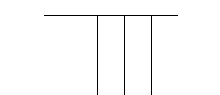
Figure 8-15: Compact Representation of an Assignment Problem

THEOREM 8.5 (Integral Property of the Assignment Problem) An op-

timal solution of the assignment problem with the requirement that x

ij

=0or 1 is

the same as an optimal solution of the linear programming problem given by (8.20),

(8.21), (8.22), and (8.23).

 Exercise 8.27 Use the integral property of the transportation problem to prove Theo-

rem 8.5.

The assignment problem can be represented compactly in an assignment array

similar to the transportation problem. See Figure 8-15 for a compact representation

ofa4× 4 example.

COROLLARY 8.6 (Number of Nonzero Basic Variables Is n) The integer

solution x to the assignment problem has exactly one x

ij

=1in every row in the

assignment array and the sum n of these x

ij

counts the number of basic variables

that are positive.

Comment: The linear program equivalent to an assignment problem has the prop-

erty that every basic solution is degenerate, since there are 2n − 1 basic variables

and exactly n basic variables must receive unit value, the remaining n − 1 basic

variables must therefore all be zero. Thus the linear program is highly degenerate.

To the best of the authors’ knowledge it is not known whether a special rule is

needed to avoid cycling. The random choice rule can be used to avoid cycling with

probability 1.

TWO ILLUSTRATIONS OF THE ASSIGNMENT PROBLEM

Example 8.17 (Prototype Assignment Problem) Suppose that we need to assign

four employees to four new tasks at the training costs shown in Figure 8-16. We set up

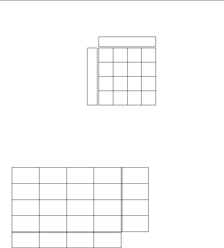
8.5 THE ASSIGNMENT PROBLEM 231

3 7 11 8

0446

0 4 10 9

0065

1234

1

2

3

4

Task

E

m

p

l

o

y

e

Figure 8-16: Training Cost Data for Assigning Employees to Tasks

3 7 11 8

0446

0 4 10 9

0065

1

1111 z =3

.

1

.

0

.

1

.

0

.

1

.

0

.

1

.

....................................................................................

.

..

.

c

1

i

4

∗

4

0

c

2

i

−

4

∗

0

c

3

i

−

0

5

∗

5

c

4

i

−

0

−

5

∗

c

5

i

−

0

−

1

c

1

j

0421

c

2

j

0421

c

3

j

−

421

c

4

j

−−

21

c

5

j

−−

2

∗

1

Figure 8-17: Initial Solution to an Assignment Problem by Vogel’s Method

Dantzig G., Thapa M. Linear programming. Vol.1. Introduction

Подождите немного. Документ загружается.