Dantzig G., Thapa M. Linear programming. Vol.1. Introduction

262 NETWORK FLOW THEORY

.

..

.

1

.

..

.

2

.

..

.

3

.

..

.

4

............................................................................................

.

............................................................................................

.

............................................................................................

.

[2,5] [4,6] [1,4]

x

o

12

=3 x

o

32

=5 x

o

34

=2

Chain ﬂow

.

..

.

1

.

..

.

2

.

..

.

3

.

..

.

4

............................................................................................

.

............................................................................................

.

............................................................................................

.

θθθ

θ Path ﬂow

.

..

.

1

.

..

.

2

.

..

.

3

.

..

.

4

............................................................................................

.

............................................................................................

.

............................................................................................

.

[2,5] [4,6] [1,4]

3+θ 5−θ 2+θ

Chain ﬂow after θ

augmentation along

the associated path

Figure 9-6: Chain Flow, θ Path Flow, θ-Flow Augmentation

THEOREM 9.5 (Flow Decomposition) Consider a network (Nd, Ac) where

the arc-capacity constraints are 0 ≤ x

ij

≤ h

ij

for (i, j) ∈Ac. Given an incoming

exogenous ﬂow of F>0, a set of ﬂows x = x

o

ij

that satisfy the capacity constraints

and conservation equations (9.6)–(9.9) can be decomposed into a vector sum of path

ﬂows from source to destination and circuit ﬂows such that the direction of these

ﬂows in any common arc (i, j) is the same as that of the directed arc (i, j) ∈Ac.

Example 9.4 (Illustration of Flow Decomposition) The Flow Decomposition The-

orem 9.5 is illustrated in Figure 9-7. The sum of the two path ﬂows and circuit ﬂow is

equal to the total ﬂow shown in Figure 9-5.

9.3 AUGMENTING PATH ALGORITHM FOR

MAXIMAL FLOW

The maximal-ﬂow problem for a network is to ﬁnd the maximum amount that can

be transferred from the source to the destination given arc-capacity constraints

l

ij

≤ x

ij

≤ h

ij

and the existence of a feasible ﬂow x = x

o

. We will also assume that

all l

ij

= 0. It is clear that solving the maximal ﬂow problem is the same as solving

the linear program

Maximize F

subject to



j∈Af (1)

x

1j

= −F,



i∈Bf (k)

x

ik

−



j∈Af (k)

x

kj

=0, for k =2,...,m− 1,



i∈Bf (m)

x

im

= F,

0 ≤ x

ij

≤ h

ij

, for all (i, j) ∈Ac.

(9.13)

9.3 AUGMENTING PATH ALGORITHM FOR MAXIMAL FLOW 263

.

..

.

1

.

..

.

2

.

..

.

4

.

..

.

6

.

...........................................................................................

.

....................................................................................

.

F =1

....................................................................................

.

F =1

1

.

..

.

............................................................................................

.

Path Flow θ =1

.

..

.

..

.

1

.

..

.

2

.

..

.

3

.

..

.

4

.

..

.

..

.

6

.

...........................................................................................

.

....................................................................................

.

F =3

....................................................................................

.

F =3

3

.

............................................................................................

.

..

.

Path Flow θ =3

.

..

.

2

.

..

.

3

.

..

.

4

.

..

.

5

...........................................................................................

.

1

11

............................................................................................

.

............................................................................................

.

Circuit Flow θ =1

Figure 9-7: Decomposition of Flow in Figure 9-5

264 NETWORK FLOW THEORY

.

..

.

1

.

..

.

2

.

..

.

3

.

..

.

4

.............................................................................

.

............................................................................................

.

............................................................................................

.

............................................................................................

.

.............................................................................

.

F =0 F =0

Figure 9-8: Augmentation Not Possible

Deﬁnition (Flow Value): The variable F , the exogenous ﬂow into the system,

is called the ﬂow value.

 Exercise 9.7 Show that by adjoining a “back ﬂow” arc (t, s), of inﬁnite capacity, joining

the destination node t to the source node s, and dropping the exogenous ﬂow equations,

the maximal ﬂow problem is equivalent to ﬁnding a feasible ﬂow in the new network that

maximizes x

ts

instead of F .

THEOREM 9.6 (Existence of a Positive Maximal Flow) In a network

with bounds 0 ≤ x

ij

≤ h

ij

for all (i, j) ∈Ac, the maximal ﬂow is positive if and

only if there exists a chain of arcs joining the source to the destination such that a

positive θ-ﬂow augmentation along the associated ﬂow path is possible.

Example 9.5 (Maximal Flow Is Zero) In Figure 9-8 we illustrate a very simple

network in which a θ-ﬂow augmentation is not possible if the ﬂow on the directed arcs

must be nonnegative. Hence the maximal ﬂow is zero.

 Exercise 9.8 Show that if the network deﬁned by (9.13) has no chains connecting the

source to the destination, the network is disconnected and the maximum ﬂow value is 0.

Show that a disconnected network does not necessarily imply that the maximal ﬂow is

zero.

THEOREM 9.7 (Existence of an Improving Flow) Consider a network

(Nd, Ac) with arc-capacities 0 ≤ x

ij

≤ h

ij

for all (i, j) ∈Ac. Given a feasible

ﬂow x = x

o

ij

with F = F

o

, a ﬂow value F>F

o

can be found if and only if there

exists a chain of arcs joining the source to the destination such that a positive θ-ﬂow

augmentation along its associated ﬂow path is possible.

Example 9.6 (Illustration of an Improving Flow) Steps to obtain an improving

ﬂow are illustrated in Figure 9-9. The numbers in brackets at the tail of each arc represent

the lower and upper bounds on the ﬂow through the arc.

COROLLARY 9.8 (Maximal Flow Condition) The ﬂow value F = F

o

is

maximal if and only if there is no chain of arcs joining the source to the destination

such that a positive θ-ﬂow augmentation along its associated ﬂow path is possible.

9.3 AUGMENTING PATH ALGORITHM FOR MAXIMAL FLOW 265

.

..

.

1

.

..

.

2

.

..

.

..

.

3

.

..

.

4

.

..

.

5

....................................................

.

............................................................................................

.

..

.

..

.

............................................................................................

.

............................................................................................

.

....................................................

.

F =3

[2,5]

[0,∞]

[4,6] [1,4]

F =3

x

o

12

=3

x

o

23

=8

x

o

34

=8

x

o

42

=5 x

o

45

=3

Initial network ﬂow

.

..

.

1

.

..

.

2

.

..

.

4

.

..

.

5

............................................................................................

.

............................................................................................

.

............................................................................................

.

[2,5] [4,6] [1,4]

x

o

12

=3 x

o

42

=5 x

o

45

=3

A chain ﬂow

.

..

.

1

.

..

.

2

.

..

.

4

.

..

.

5

............................................................................................

.

............................................................................................

.

............................................................................................

.

θθθ

θ Path ﬂow

.

..

.

1

.

..

.

2

.

..

.

4

.

..

.

5

............................................................................................

.

............................................................................................

.

............................................................................................

.

[2,5] [4,6] [1,4]

3+θ 5−θ 3+θ

The chain ﬂow after θ

augmentation along

the associated path

.

..

.

1

.

..

.

2

.

..

.

3

.

..

.

4

.

..

.

5

....................................................

.

............................................................................................

.

..

.

..

.

............................................................................................

.

............................................................................................

.

....................................................

.

F =4

[2,5]

[0,∞]

[4,6] [1,4]

F =4

x

o

12

=4

x

o

23

=8

x

o

34

=8

x

o

42

=4 x

o

45

=4

Improved network ﬂow

obtained by setting θ =1

Figure 9-9: Finding an Improved Flow

266 NETWORK FLOW THEORY

 Exercise 9.9 Show that the improving ﬂow in Example 9.6 results in a maximal ﬂow

for the network.

 Exercise 9.10 Prove Corollary 9.8.

Instead of adjusting ﬂows in a network-ﬂow problem, it is convenient to adjust

the arc capacities so that all the existing ﬂows x

o

ij

are converted to zero and an im-

proving ﬂow is found in this adjusted-capacity network. After ﬁnding the improving

ﬂow, the arc capacities are again adjusted so that θ improvements are converted

to zero, and so on, iteratively. A ﬁnal step notes the diﬀerence between the ﬁnal

adjusted capacity and the original capacity on an arc, and this diﬀerence is x

∗

ij

, the

maximal ﬂow solution.

Deﬁnition (Adjusted-Capacity Network): Given any existing ﬂow x = x

0

ij

on a

network (Nd, Ac), the adjusted-capacity network is a network that is computed

as follows. Subtract existing arc-ﬂows x

o

ij

from the upper bound h

ij

on arc-

capacity to obtain a new upper bound

¯

h

ij

= h

ij

−x

o

ij

on the arc capacity. Add

a reverse arc (j, i) with an upper bound

¯

h

ji

= x

o

ij

on arc capacity; if x

o

ij

=0,

the reverse arc (j, i) may be omitted.

Example 9.7 (Construction of an Adjusted-Capacity Network) In Figure 9-10

we illustrate how to obtain an adjusted-capacity network from a network with initial ﬂows.

The direction of the existing ﬂow is shown by the arrows, and the ﬂow values are shown

as numbers approximately halfway on each arc. It is assumed that each pair of nodes has

two arcs connecting it. The capacity on the arc from node i to node j is shown at the

tail of the arc; i.e., near node i. In the ﬁgure, on the line joining node 1 and node 2, the

number 4 near node 1 is the arc capacity for arc (1, 2) and the number 0 near node 2 is

the arc capacity for arc (2, 1). In Figure 9-10(a), an initial exogenous ﬂow of F =5is

assumed. In Figure 9-10(b) we have created an adjusted-capacity network by converting

the existing ﬂows to zero as discussed above.

Theorem 9.7 is a theoretical basis for the Ford-Fulkerson Augmenting Path Al-

gorithm (also due independently to Elias, Feinstein, and Shannon). We shall ﬁrst

illustrate the algorithm through an example.

Example 9.8 (Illustration of the Augmenting Path Algorithm) Consider the

network displayed in Figure 9-11(a) with the capacities of the forward and reverse arcs

as shown by capacities on both ends of the arcs. Notice that the arc connecting nodes 2

and 3 has a capacity of 1 along the arc, (2, 3) and a capacity of 2 along the arc (3, 2); i.e.,

the arc joining nodes 2 and 3 is undirected and has been replaced by two arcs (2, 3) and

(3, 2). Noting that there are no existing ﬂows, we start the algorithm by setting F =0

and ﬁnding an augmenting path such as (1, 3), (3, 2), and (2, 4) with arc capacities 2, 2,

and 2 respectively. Thus the improving ﬂow θ through this path is 2, and F =0+2. The

capacities are then adjusted by subtracting θ = 2 from the tail of the forward arcs along

the path and adding θ = 2 to the tail of the reverse arcs along the path to generate the

next adjusted-capacity network, shown in Figure 9-11(b).

9.3 AUGMENTING PATH ALGORITHM FOR MAXIMAL FLOW 267

.

..

.

1

.

..

.

2

.

..

.

3

.

..

.

4

.

2

3

1

2

3

....................................................

.

F

o

=5

....................................................

.

F

o

=5

.

4

2

02

1

03

2

0

(a)Network with initial nonzero ﬂow

.

..

.

1

.

..

.

2

.

..

.

3

.

..

.

4

.

1

0

30

0

20

3

2

3

(b)Associated network with zero ﬂows.

Figure 9-10: Construction of an Adjusted-Capacity Network

In the new network there is only one augmenting path, namely the one with arcs

(1, 2), (2, 3), and (3, 4) with capacities 4, 3, and 3 respectively. Therefore the improving

ﬂow for this iteration is θ = 3, and thus F =2+θ = 5. Notice how the ﬂow in arc (2, 3)

more than counteracts the ﬂow of the previous iteration on arc (3, 2). Adjusting the arc

capacities on the augmenting path by θ = 3, we get the adjusted-capacity network shown

in Figure 9-11(e).

No augmenting path exists, and therefore, by Theorem 9.7, the solution is optimal.

From the arc capacities in the adjusted-capacity network of Figure 9-11(e) we compute

the diﬀerence between original arc-capacities, shown in Figure 9-11(e), and the ﬁnal arc-

capacities shown in Figure 9-11(e) to obtain the ﬁnal maximal ﬂow solution, shown in

Figure 9-11(f).

Algorithm 9.1 (Augmenting Path) In general, we ﬁrst create an adjusted-capacity

network by adding to each arc (i, j) that does not have a reverse arc (j, i) an arc (j, i)

with capacity

¯

h

ji

= 0 (the capacities on the arcs corresponding to the original network are

relabeled as

¯

h

ij

). Set the ﬂow F = 0 in this adjusted system. The original network with

arc-capacities h

ij

is set aside until the termination of the algorithm, when its ﬂows are set

to the optimal ﬂows.

1. Using any θ-ﬂow augmenting search procedure, try to ﬁnd an augmenting path for

the current adjusted-capacity network. If no such path exists, stop with the updated

ﬂow value F being optimal and the optimal arc-ﬂows determined by

x

∗

ij

=

¯

h

ij

− h

ij

for each arc in the original network.

2. Determine θ equal to the minimum capacity for the augmenting path in the current

adjusted-capacity network:

θ = min

(i,j)∈AP

¯

h

ij

,

where AP is the augmenting path. Set F ← F + θ.

268 NETWORK FLOW THEORY

.

..

.

1

.

..

.

2

.

..

.

3

.

..

.

4

.

4

2

02

1

03

2

0

(a)Initial Network.

.

..

.

1

.

..

.

2

.

..

.

3

.

..

.

4

.

θ=2

.............................................................................

.

θ=2

....................................................

.

θ=2

.

4

2

02

1

03

2

0

(b)Iteration 1: Initiating path ﬂow

.

..

.

1

.

..

.

2

.

..

.

3

.

..

.

4

.

4

0

00

3

23

0

2

0

(c)Adjusted arc capacities.

.

..

.

1

.

..

.

2

.

..

.

3

.

..

.

4

.

θ=3

....................................................

.

θ=3

....................................................

.

θ=3

.

4

0

00

3

23

0

2

0

(d)Iteration 2: Adjusted arc capacities

and an augmenting path.

.

..

.

1

.

..

.

2

.

..

.

3

.

..

.

4

.

1

0

30

0

20

3

2

3

(e)Iteration 3: Final adjusted arc

capacities, no additional path

ﬂow possible.

.

..

.

1

.

..

.

2

.

..

.

3

.

..

.

4

.

2

1

23

3

....................................................

.

max F =5

....................................................

.

F =5

.

4

2

02

1

03

2

0

(f) Iteration 4: Maximal ﬂow as the sum

of all the possible path ﬂows.

Figure 9-11: Illustration of the Augmenting Path Algorithm to Find Maximal Flow

9.3 AUGMENTING PATH ALGORITHM FOR MAXIMAL FLOW 269

3. For each directed arc (i, j) of the adjusted-capacity network along the augmenting

path, adjust the arc-capacity to be

¯

h

ij

←

¯

h

ij

− θ,

¯

h

ji

←

¯

h

ji

+ θ

to determine the next adjusted-capacity network.

4. Go to Step 1.

Note that the algorithm only modiﬁes the arc capacities in the adjusted-capacity

network and not its arc ﬂows. The optimal arc ﬂows x

∗

ij

for the original network

are actually the sums of the individual path ﬂows encountered during the solution

process; hence these could have been determined by adjusting the ﬂows x

ij

at the

same time that the arc capacities h

ij

were adjusted in Step 3. However, a simpler

way is to obtain them from the ﬁnal adjusted-capacity network by comparing the

ﬁnal arc capacities with the initial assigned arc capacities. If for arc (i, j) the ﬁnal

arc capacity

¯

h

ij

is less than the initially assigned arc capacity h

ij

, then arc (i, j)

has a ﬂow equal to the diﬀerence; i.e., x

ij

= h

ij

−

¯

h

ij

.

 Exercise 9.11 Modify Algorithm 9.1 if the initial feasible ﬂow vector x = x

o

=0is

given.

 Exercise 9.12 Modify Algorithm 9.1 so that instead of modifying the arc capacities we

update the ﬂows directly. In this case we check for augmenting paths such that the arcs

in the path can be traversed in the direction of the arc if the ﬂow is less than the upper

bound, and in the reverse direction if the ﬂow is greater than the lower bound.

Starting with a feasible solution x

ij

= x

o

ij

= 0 for all (i, j) ∈Ac, Algorithm 9.1,

regardless of the augmenting path procedure, is guaranteed to solve the maximal

ﬂow problem in a ﬁnite number of augmenting ﬂow steps provided that the arc ca-

pacities are either integers or rational numbers (see Theorem 9.9 and Corollary 9.10).

In the event that the ﬂow capacities are not rational numbers, the algorithm may

sometimes require an inﬁnite number of steps to converge. However, even if the

ﬂow capacities are not rational, the use of a procedure for ﬁnding an augmenting

path, called the Breadth-First Unblocked Search procedure (to be discussed later), is

guaranteed by the Edmonds-Karp Theorem 9.11 to solve the maximal ﬂow problem

within mn/2 ﬂow augmenting steps, where m is the number of nodes and n is the

number of arcs.

THEOREM 9.9 (Finite Termination with Integer Capacities) If the arc

capacities are all integers and a ﬁnite maximal ﬂow exists, then Algorithm 9.1 will

construct only a ﬁnite number of path ﬂows whose algebraic sum is the maximal

ﬂow.

270 NETWORK FLOW THEORY

.

..

.

1

.

..

.

2

.

..

.

3

.

..

.

4

.......................................

.

.......................................

.

..

.

..

.

..

.

1000

0

1

1000

0

1000

0

Figure 9-12: Large Number of Iterations of Algorithm 9.1

COROLLARY 9.10 (Finite Termination with Rational Capacities) If

the arc capacities are all rational numbers and a ﬁnite maximal ﬂow exists, then

Algorithm 9.1 will construct only a ﬁnite number of path ﬂows whose algebraic sum

is the maximal ﬂow.

The next example demonstrates that it is possible to choose augmenting paths

such that the algorithm takes a very large number of iterations to converge.

Example 9.9 (Large Number of Iterations of the Augmenting Path Algorithm)

Consider the network in Figure 9-12. It may seem that the greater the number of arcs in

the chosen augmenting path at each iteration, the sooner the sum of the augmenting path

ﬂows will use up capacity of the arcs and terminate with maximal ﬂow. However if we

apply this strategy to the network shown in Figure 9-12, we would choose path (1, 2, 3, 4)

on odd iterations and (1, 3, 2, 4) on even iterations and ﬁnd that Algorithm 9.1 takes 2,000

iterations to converge! If the capacity on each arc with capacity of 1,000 is changed to a

capacity of a trillion, the algorithm would require two trillion iterations. If the capacity

restrictions on the arcs with capacities of a 1,000 are dropped, the algorithm would never

terminate. Notice that if at each iteration we had chosen instead the augmenting path

with the fewest number of arcs, the algorithm would have terminated in two iterations!

 Exercise 9.13 Create a network for which the augmenting path algorithm chooses at

each iteration an augmenting path with the largest number of arcs, and solves the problem

faster than one that chooses an augmenting path with the smallest number of arcs.

The following example demonstrates that if the capacities are irrational numbers

then it is possible that the maximal ﬂow Algorithm 9.1 may never terminate even

if all the capacities are all ﬁnite.

Example 9.10 (Inﬁnitely Many Iterations of the Augmenting Path Algorithm)

Consider the network in Figure 9-13 with source node 1, destination node 8, and bounds

on arcs

0 ≤ x

23

≤ h,

0 ≤ x

47

≤ 1,

0 ≤ x

57

≤ h,

0 ≤ x

ij

≤∞,

where h =



−1+

√

5



/2 is the golden ratio. It turns out that the algorithm will go

through an inﬁnite sequence of iterations τ shown in Table 9-1 if one chooses cyclically for

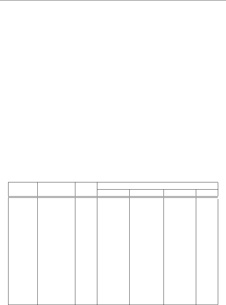
9.3 AUGMENTING PATH ALGORITHM FOR MAXIMAL FLOW 271

.

..

.

1

.

..

.

2

.

..

.

3

.

..

.

4

.

..

.

5

.

..

.

6

.

..

.

7

.

..

.

8

....................................................

.

....................................................

.

..

.

..

.

.....................................................................................................................

.

.....................................................................................................................

.

.....................................................................................................................

.

.....................................................................................................................

.

h

1

h

Figure 9-13: Inﬁnite Number of Iterations of Algorithm 9.1

Augmenting Path Resulting Arc Flow (on relevant arcs)

Iteration Path Flow x

23

x

47

x

57

x

76

1 1,2,3,4,7,8 h h h =1−h

2

0 0

2 1,3,2,4,7,6,8 h

2

h − h

2

1 0 h

2

3 1,2,3,5,7,8 h

2

h 1 h

2

h

2

4 1,3,2,5,7,4,8 h

3

h − h

3

1 − h

3

h h

2

5 1,2,3,6,7,8

h

3

h 1 − h

3

h h

4

6 1,3,2,6,7,5,8 h

4

h − h

4

1 − h

3

h − h

4

0

.

6τ +1 1,2,3,4,7,8 h

3τ+1

h 1 − h

3τ+2

h − h

3τ+1

0

6τ +2 1,3,2,4,7,6,8 h

3τ+2

h − h

3τ+2

1 h − h

3τ+1

h

3τ+2

6τ +3 1,2,3,5,7,8 h

3τ+2

h 1 h −h

3τ+3

h

3τ+2

6τ +4 1,3,2,5,7,4,8 h

3τ+3

h − h

3τ+3

1 − h

3τ+3

h h

3τ+2

6τ +5 1,2,3,6,7,8 h

3τ+3

h 1 − h

3τ+3

h h

3τ+4

6τ +6 1,3,2,6,7,5,8 h

3τ+4

h − h

3τ+4

1 − h

3τ+3

h − h

3τ+4

0

.

Table 9-1: Inﬁnite Number of Iterations of Algorithm 9.1

Dantzig G., Thapa M. Linear programming. Vol.1. Introduction

Подождите немного. Документ загружается.