Davim J.P. Tribology for Engineers: A Practical Guide
Подождите немного. Документ загружается.

1
2
3
4
5
6
7
8
9
10
10
1
2
3
4
5
6
7
8
9
20
20
1
2
3
4
5
6
7
8
9
30
30
1
2
3
34R
34R
8
Tribology for Engineers
Roughness is usually characterized by either of the two
statistical height descriptors advocated by the International
Standardization Organization (ISO) and the American
National Standards Institute (ANSI) (Anonymous, 1985).
These are CLA (Centre-line average, R
a
) and RMS (Root
mean square, R
q
). Two other statistical height descriptors are
rarely used – skewness (Sk) and kurtosis (K).
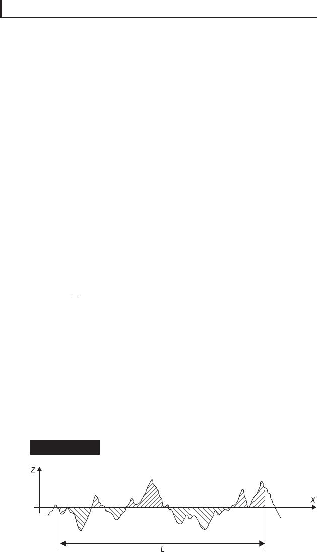
1.3.1 Centre line average (CLA)
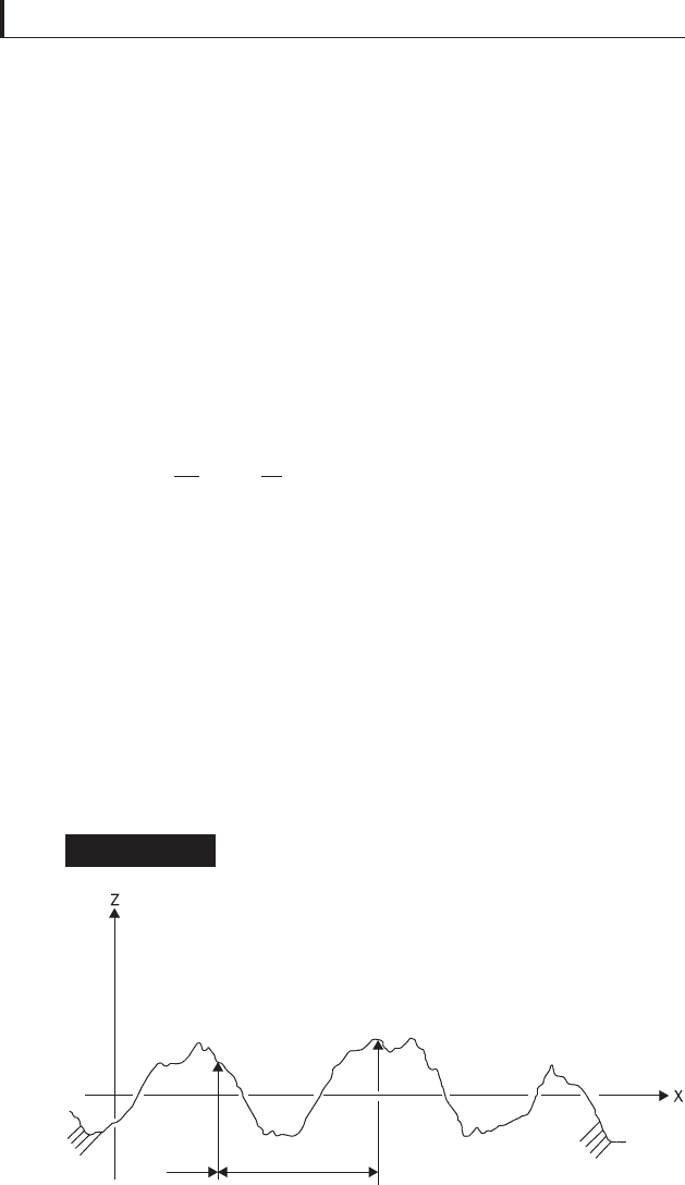
It is defi ned as the arithmetic mean deviation of the surface
height from the mean line through the profi le. It is also
termed as average roughness (symbol R
a
). Here the mean
line is defi ned so as to have equal areas of the profi le above
and below it. It may also be defi ned by the equation
R
a
1
∫
L
0
Z(x)
dx
[1.1]
L
where Z(x) is the height of the surface above the mean line at
a distance x from the origin and L is the measurement length
of the profi le (Fig. 1.4). The R
a
value of a surface profi le
depends on its manufacturing method and some typical
R
a
(
μ
m) values are: rough casting – 10, coarse machining – 3
to 10, fi ne machining – 1 to 3, grinding and polishing – 0.2
Centre line average of a surface over sampling
length L
Figure 1.4

1
2
3
4
5
6
7
8
9
10
10
1
2
3
4
5
6
7
8
9
20
20
1
2
3
4
5
6
7
8
9
30
30
1
2
3
34R
34R
9
Surface topography
to 1 and lapping – 0.02 to 0.4. The disadvantage of using the
R
a
value is that this fails to distinguish between a sharp spiky
profi le and a gently wavy profi le. It is possible for surfaces of
widely varying profi les with different frequencies and shapes
to have the same R
a
value (Fig. 1.5).
Various surface profi les having the same
R
a
value
Figure 1.5
1
2
3
4
5
6
7
8
9
10
10
1
2
3
4
5
6
7
8
9
20
20
1
2
3
4
5
6
7
8
9
30
30
1
2
3
34R
34R
10
Tribology for Engineers
1.3.2 RMS roughness
This parameter represents the standard deviation of the
distribution of the surface heights, so it is an important
parameter to describe the surface roughness by statistical
methods. This parameter is more sensitive than the arithmetic
average height (R
a
) to large deviation from the mean line. It
is defi ned as the root mean square deviation of the profi le
from the mean line. It is denoted by the symbol R
q
. The
mathematical defi nition and the digital implementation of
this parameter are as follows:
R
q
1
∫
L
0
[Z(x)]
2
dx
[1.2]
L
The RMS mean line is the line that divides the profi le so that
the sum of squares of the deviations of the profi le height
from it is equal to zero.
1.3.3 Skewness and kurtosis
The skewness is a measure of the departure of a distribution
curve from its symmetry and kurtosis is the measure of the
bump on a distribution curve. The skewness and kurtosis in
the normalized form may also be given as
Sk
1
∫
L
0
Z
3
dx
[1.3]
σ
3
L
and
K
1
∫
L
0
Z
4
dx
[1.4]
σ
4
L
where
σ
is the standard deviation of the distribution of
asperity heights.

1
2
3
4
5
6
7
8
9
10
10
1
2
3
4
5
6
7
8
9
20
20
1
2
3
4
5
6
7
8
9
30
30
1
2
3
34R
34R
11
Surface topography
1.4 Statistical aspects
Another way of statistical treatment of a surface profi le is to
consider the probability distribution function of the height
Z. The same is denoted by P(Z) or
φ
(Z) and is obtained by
plotting the number of occurrences of a particular value of
Z in the data against the value of Z and normalizing the best
fi t curve to the data so that the total area enclosed by the
distribution curve is unity. Thus it is given as
∫
∞
∞
φ
(Z)dZ 1 [1.5]
The distribution function for most real surfaces is generally
in the form of a ‘bell-shaped’ curve and can be described
approximately by a Gaussian distribution given as
Symbol Name Defi nition
R
t
Peak-to-valley height Separation of highest peak and
lowest valley
R
p
Peak-to-mean height Separation of highest peak and
mean line
R
v
Mean-to-valley height Separation of mean line and lowest
valley
R
z
(DIN) Average peak-to-valley
height
Average of single R
t
values over
fi ve adjoining sampling lengths
R
z
(ISO) Ten point height Separation of average of fi ve highest
peaks and fi ve lowest valleys within
single sampling length
R
pm
Average peak-to-mean
height
Separation of average of fi ve
highest asperities and mean line
Defi nitions of a few surface roughness
parameters
Table 1.1
Some more extreme value height descriptors are also used
as defi ned in Table 1.1.

1
2
3
4
5
6
7
8
9
10
10
1
2
3
4
5
6
7
8
9
20
20
1
2
3
4
5
6
7
8
9
30
30
1
2
3
34R
34R
12
Tribology for Engineers
φ
(Z)
1
exp( Z
2
/2
σ
2
) [1.6]
σ
√2
––
π
–
where
σ
is the standard deviation of the distribution.
The shape of the distribution function may be quantifi ed
by means of the moments of the distribution. The nth
moment of the distribution m
n
is defi ned as
m
n
∫
∞
∞
Z
n
φ
(Z)dZ [1.7]
The fi rst moment m
1
represents the mean line. The mean line
is so located that m
1
is equal to zero. Then the second moment
m
2
is equal to
σ
2
, the variance of the distribution. From
defi nition of R
q
it is seen that R
q
=
σ
. It can also be shown that
R
q
/R
a
for a Gaussian distribution comes out to be nearly 1.25.
The third moment m
3
in normalized form gives the skewness,
Sk (= m
3
/
σ
3
), which provides some measure of the departure
of the distribution from symmetry. For a symmetrical
distribution like Gaussian distribution, Sk = 0. The fourth
moment m
4
in normalized form gives the kurtosis (= m
4
/
σ
4
),
which is a measure of the sharpness of the peak of the
distribution curve. For Gaussian distribution, K = 3. K > 3
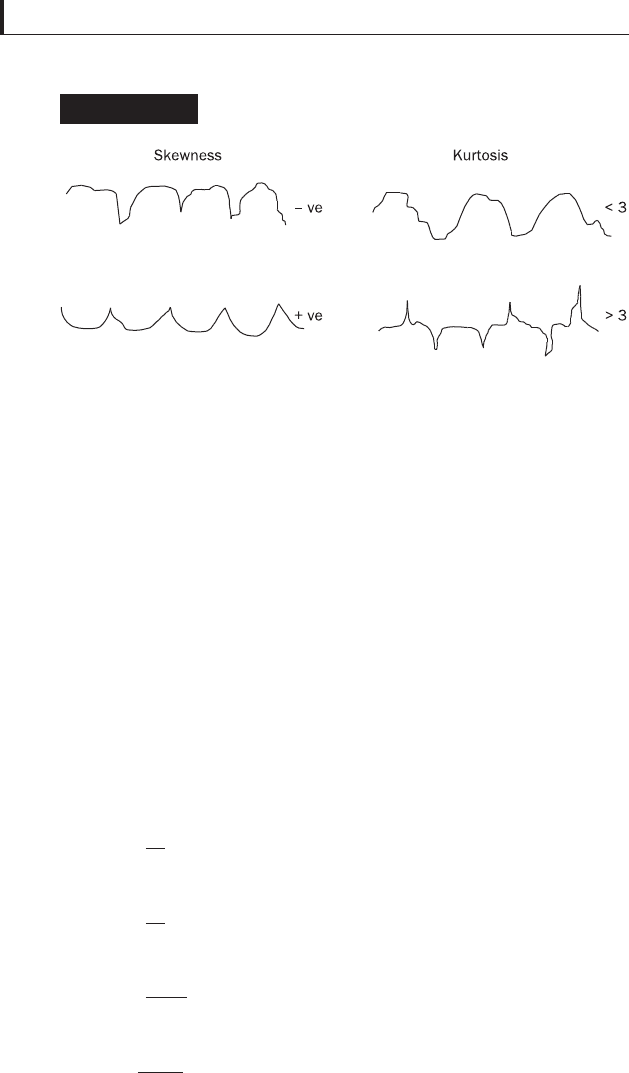
means peak sharper than Gaussian and vice versa. Figure 1.6
shows a Gaussian distribution function as well as distribution
functions with various skewness and kurtosis values, while
Fig. 1.7 shows examples of surfaces with different skewness
and kurtosis values. A surface with a Gaussian distribution
has peaks and valleys distributed evenly about the mean:
■
A surface with positive value of skewness has a wider
range of peak heights that are higher than the mean.
■
A surface with negative value of skewness has more peaks
with heights close to the mean as compared to a Gaussian
distribution.
■
A surface with very low kurtosis has more local asperities
above the mean as compared to a Gaussian distribution.

1
2
3
4
5
6
7
8
9
10
10
1
2
3
4
5
6
7
8
9
20
20
1
2
3
4
5
6
7
8
9
30
30
1
2
3
34R
34R
13
Surface topography
■
A surface with very high kurtosis has fewer asperities
above the mean.
In practice many engineering surfaces follow symmetrical
Gaussian height distribution (Whitehouse, 1994). Generally,
for most engineering surfaces the height distribution is
(a) Probability density functions for random
distribution with different skewness; (b)
symmetrical distributions (zero skewness) with
different kurtosis
Figure 1.6
1
2
3
4
5
6
7
8
9
10
10
1
2
3
4
5
6
7
8
9
20
20
1
2
3
4
5
6
7
8
9
30
30
1
2
3
34R
34R
14
Tribology for Engineers
Gaussian at the high end and non-Gaussian at the lower end,
the bottom 1–5% of the distribution (Williamson, 1968).
Many common machining processes produce surfaces with
non-Gaussian distribution: turning, shaping and electro
discharge machining produce positively skewed surfaces;
milling, honing, grinding and abrasion processes produce
surfaces with negative skewness but high kurtosis values.
Non-Gaussian surfaces are modelled using the well-known
Weibull distribution and Pearson system of frequency curves.
For a digitized profi le of length L with heights Z
i
, i = 1 to
N, at a sampling interval h = L/(N – 1), where N represents
the number of measurements, average height parameters are
given as
R
a
1
兺
N
i1
Z
i
m
[1.8]
N
σ
2
1
兺
N
i1
(Z
i
m)
2
[1.9]
N
Sk
1
兺
N
i1
(Z
i
m)
3
[1.10]
σ
3
N
K
1
兺
N
i1
(Z
i
m)
4
[1.11]
σ
4
N
Schematic illustration for random functions with
various skewness and kurtosis values
Figure 1.7
1
2
3
4
5
6
7
8
9
10
10
1
2
3
4
5
6
7
8
9
20
20
1
2
3
4
5
6
7
8
9
30
30
1
2
3
34R
34R
15
Surface topography
and
m
1
兺
N
i1
Z
i
[1.12]
N
It is important to note here that all these statistical parameters
are based on random data and hence they are subject to
random statistical variations. They may not represent the
true functional property of the surface in consideration.
Moreover, none of these contain information on the horizontal
or spatial distribution. There are a number of parameters
that serve the description in spatial distribution. A few are
described here.
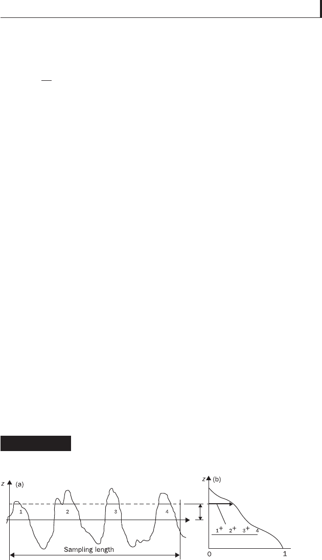
1.4.1 Abbott bearing area curve
Sometimes it is required to estimate the proportion of the
nominal area between two contacting surfaces that are in
real contact. This is displayed on a curve known as the
Abbott and Firestone bearing area curve (Abbott and
Firestone, 1933). Figure 1.8 shows the construction of such
a bearing area curve. A line parallel to the mean line is drawn
at some height d and then the sum of all the intercepts along
this line is expressed as a proportion of the total measurement
length, given as (a
1
+ a
2
+ …)/L. This actually gives a bearing
Construction of the Abbott bearing area curve
from the topography of a surface: (a) surface
profi le; (b) bearing area curve
Figure 1.8
aaa
L
L
d
x
a
aaaa
1
2
3
4
5
6
7
8
9
10
10
1
2
3
4
5
6
7
8
9
20
20
1
2
3
4
5
6
7
8
9
30
30
1
2
3
34R
34R
16
Tribology for Engineers
length. If the surface be isotropic, i.e., has no defi nite
directional roughness, then the bearing length and bearing
area are numerically equal.
1.4.2 Autocorrelation function (ACF)
The autocorrelation function (ACF) provides some
information about the distribution of hills and valleys across
the surface. The normalized ACF,
ρ
(
β
), of a profi le Z(x) is
defi ned as
ρ
(
β
)
1
{
lim
1
∫
L
0
Z(x).Z(x
β
)dx
}
[1.13]
σ
2
L→∞
L
L being the sampling length and
β
the displacement along the
surface (Fig. 1.9). When
β
is zero, the value of the normalized
ACF
ρ
(0) is a maximum and equal to unity. As
β
tends to
infi nity, the extent of correlation decreases and
ρ
(
β
) tends to
zero. If
ρ
(
β
) is plotted against
β
, the curve decays from a value
of unity to zero asymptotically at large values of
β
. For many
real surfaces the ACF may be approximated by an exponential
decay function. The form of the decay curve provides some
Z(X)
Z(X + b )
X
b
Graphical representation of the autocorrelation
function
Figure 1.9
1
2
3
4
5
6
7
8
9
10
10
1
2
3
4
5
6
7
8
9
20
20
1
2
3
4
5
6
7
8
9
30
30
1
2
3
34R
34R
17
Surface topography
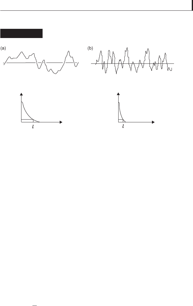
information on the horizontal distribution of roughness.
Sometimes a correlation length l is defi ned as the value of
β
at
which
ρ
(
β
) equals 0.1. The value of this l is signifi cantly
higher in the case of an open texture surface than in a closed
one (Fig. 1.10). It is suggested that the simple exponential
decay function given by
ρ
(
β
) = exp (–2.3
β
/l) is a good fi t for
many surfaces with randomness.
1.4.3 Power spectral density function (PSDF)
The power spectral density function P(
ω
) provides direct
information about the spatial frequencies present in the
profi le. Particularly in the case of machined surfaces, it
separates any strong surface periodicity resulting from the
machining process. It is obtainable from the Fourier cosine
transform of the autocorrelation function, given by
P(
ω
)
2
∫
∞
0
ρ
(
β
)cos(
ωβ
)d
β
[1.14]
π
In some modern profi lometers, automatic computation of
ACF and PSDF is possible.
Surface textures and their autocorrelation
functions
Figure 1.10
r(b ) r(b )