Edelstein-Keshet L. Mathematical Models in Biology
Подождите немного. Документ загружается.

156
Continuous Processes
and
Ordinary
Differential
Equations
(a)
Find
the
values
of c1 and c
2
by
solving
the
above.
For
questions
(b)
through
(e) find the
solution
of the
differential
equation subject
to
the
specified initial condition.
19.
When
A1 = Az = A, one
solution
of
equation (34)
is
To find
another solution (that
is not
just
a
constant multiple
but is
linearly
inde-
pendent
of the
above
solution),
consider
the
assumption
Find
first and
second
derivatives,
substitute into equation (34),
and
show that
v(t)
= t.
Conclude that
the
general solution
is
20. If
Ai.a
= a ± bi are
complex conjugate eigenvalues,
the
complex
form
of the
solutions
is
Use the
identity
and
consider
Reason that these
are
also solutions
by
linear superposition
and
thus show that
a
real-valued solution
(as in
Section 4.8)
can be
defined.
21. (a)
Show that system (40a,
b) can be
reduced
to
equation (41)
by
eliminating
one
variable.
[Hint:
differentiate both sides
of
(40a)
first, and
then make
two
other substitutions.]
(b)
Once x(t)
is
found
[see equation (42a)], y(t)
can be
found
from
(40a)
by
setting
Determine y(t)
in
terms
of the
expressions
in
(42a).
(c)
Conclude that
in
vector
form
the
solution
can be
written
as
An
Introduction
to
Continuous
Models
157
22. In the
following exercises
find the
general solution
to the
system
of
equations
dx/dt
= Ax,
where
the
matrix
A is as
follows:
23. For
problem
22(a-f)
write
out the
system
of
equations
Then eliminate
one
variable
to
arrive
at a
single second-order equation, using
the
method given
in
problem
21.
Find
the
characteristic
equation
and
solve
for
the
eigenvalues
of the
equation. Find solutions
for
x\(t)
and
x
2
(t).
24.
Consider
the
nth-order linear ordinary
differential
equation
Show that
by
assuming solutions
of the
form
one
obtains
a
characteristic equation that
is an
nth-order polynomial.
5. In
this problem
we
write
equations
to
model
the
continuous chemotherapy
de-
scribed
in
Section 4.11.
(a)
Assume that
the
effect
of the
drug
on
mortality
of
tumor
cells
is
given
by
Michaelis-Menten kinetics
[as in
equation (15)]
and
that
the
drug
is re-
moved
from
the
site
at the
rate
u.
Suggest equations
for the
tumor cell
population
N and the
drug concentration
C,
assuming that tumor
cells
grow
exponentially.
(b)
Carry
out
dimensional analysis
of
your equations
and
indicate which
di-
mensionless
combinations
of
parameters
are
important.
(c)
Determine whether
the
system admits steady-state solutions,
and if so,
what
their stability properties are.
(d)
Interpret your results
in the
biological context.
(e) A
solid tumor usually grows
at a
declining rate because
its
interior
has no
access
to
oxygen
and
other necessary substances that
the
circulation sup-
plies. This
has
been modeled empirically
by the
Gompertz growth law,
y
is the
effective tumor growth rate, which will
decrease
exponentially
by
this assumption. Show that equivalent
ways
of
writing
this
are
158
Continuous Processes
and
Ordinary
Differential
Equations
[Hint:
use the
fact
that
(f)
Use the
Gompertz
law to
make
the
model equations more
realistic.
As-
sume
that
the
drug causes
an
increase
in a as
well
as
greater tumor mor-
tality.
26.
Insulin-glucose regulation. Equations (84a,b)
due to
Bolie (1960)
are a
simple
model
for
insulin-mediated glucose homeostasis.
The
following questions
are a
guide
to
investigating this model.
(a)
When neither component
is
injected
in
normal, healthy individuals,
the
blood
glucose
and
insulin
levels
are
regulated
to
within
fairly
restricted
concentration ranges. What does this imply about equations (84a,
b)?
(b)
Explain
the
appearance
of the
factor
V on the LHS of
equations (84a,
b).
What
are the
dimensions
of the
functions
Fi, F
2
, F
3
, and F4!
(c)
Bolie defines
XQ
and
YQ
as the
mean equilibrium levels
of
insulin
and
glu-
cose
when none
is
being injected into
the
body. What equations
do
XQ
and
YQ
satisfy?
(d)
Consider
the
following
four
parameters:
[Partial derivatives
are
evaluated
at
(XQ,
YQ).]
Interpret what these represent
and
comment
on the
fact
that these
are as-
sumed
to be
positive constants.
(e)
Suppose that
i = G = 0, but
that
at
time
t = 0 a
rapid ingestion
of
glu-
cose
followed
by a
single
insulin injection changes
the
internal concen-
trations
to
where
x', y' are
small compared
to
XQ,
Y
Q
.
Discuss what
you
expect
to
happen
and how it
depends
on the
parameters
a, j8, y, and 5.
(f)
By
extrapolating empirical data
for
canines
to the
body mass
of a
human,
Bolie suggests
the
values
Are
these values consistent with
a
stable equilibrium?
27. The
following equations were suggested
by
Bellomo
et al.
(1982)
as a
model
for
the
glucose-insulin
(g, i)
hormonal system.
An
Introduction
to
Continuous
Models
159
The
coefficients
K
it
K
g
, K
s
, K
ht
K
0
are
constants whose exact
definitions
may
be
ignored
in
this problem.
(a)
Suggest
an
interpretation
of the
terms
in
these equations.
(b)
Explore
the
steady state(s)
and
stability properties
of
this system
of
equa-
tions.
Note:
For a
more extended project,
the
problem
can be
extended
to a
full
re-
port
or a
class presentation based
on
this model.
28. A
model
due to
Landahl
and
Grodsky
(1982)
for
insulin
secretion
is
based
on
the
assumption that there
are
separate storage
and
labile compartments,
a
pro-
visionary factor,
and a
signal
for
release. They
define
the
following
variables:
G —
glucose concentration,
X
=
moiety
formed
from
glucose
in
presence
of
calcium ions Ca
++
,
P
=
provisionary quantity required
for
insulin production,
Q =
total amount
of
insulin available
for
release
= CV,
where
C is its
concentration
and V is the
volume,
5 =
secretion rate
of
insulin,
/ =
concentration
of an
inhibitory quantity.
(a) The
following equation describes
the
amount
of
insulin available
for re-
lease:
where
k+, k- and y are
constant
and C
s
is the
concentration
in the
storage
compartment
(of
volume V
s
), assumed constant. Explain
the
terms
and
assumptions made
in
deriving
the
equation,
(b)
Show that another
way of
expressing part
(a) is
How
do H, y', and Q
0
relate
to
parameters which appear above?
(c) An
equation
for the
provisional factor
P is
given
as
follows:
where
/'•(G)
is
just some
function
of G
(e.g.,
PooG)
= G).
Explain what
has
been assumed about
P.
(d) The
inhibitory entity
/ is
assumed
to be
produced
at the
rate
where
B is a
rate constant
and
AT
is a
proportionality constant. Explain
this equation.
160
Continuous
Processes
and
Ordinary
Differential
Equations
Figure
for
problem
29.
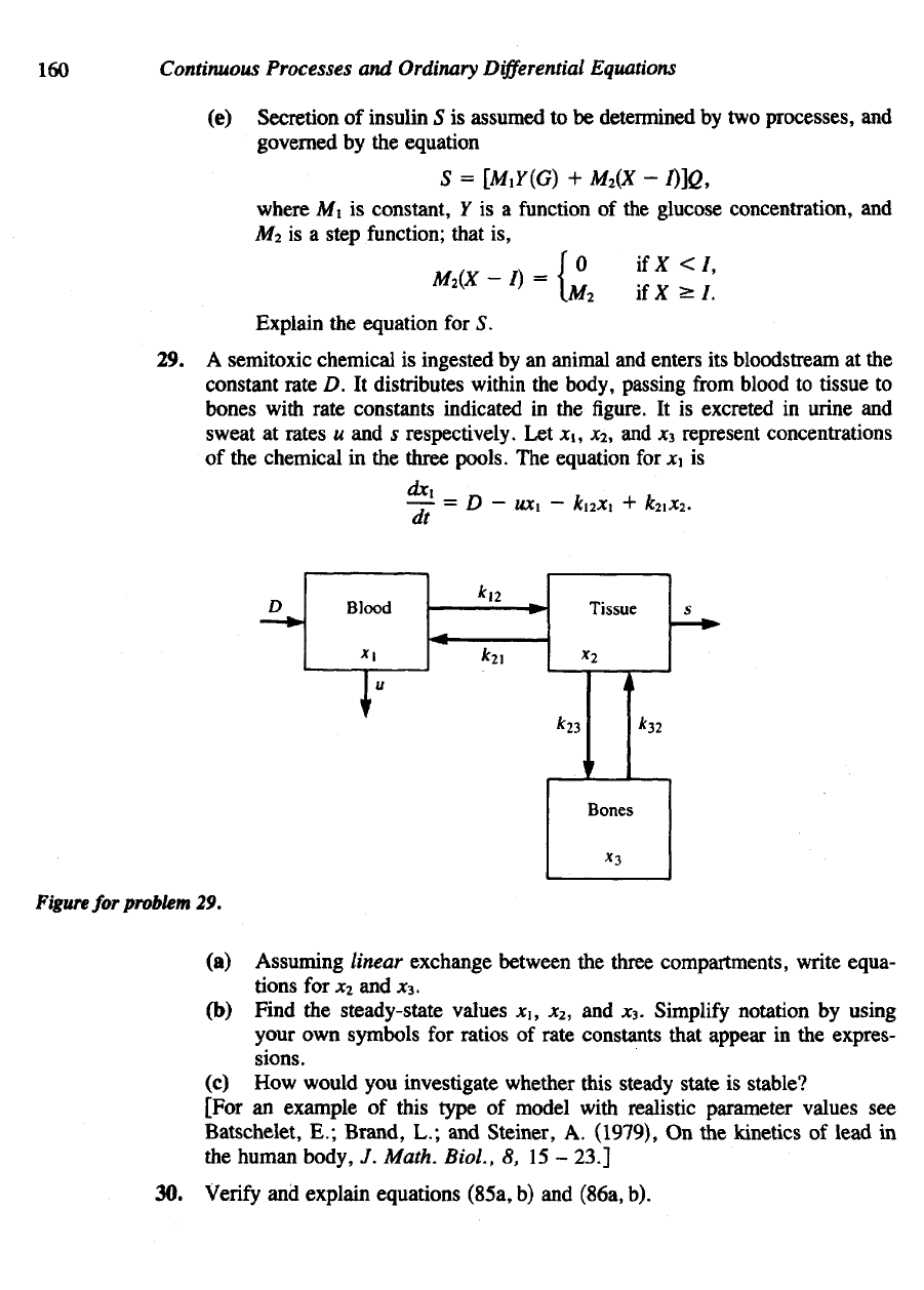
(a)
Assuming linear exchange between
the
three compartments, write equa-
tions
for x2 and x3.
(b)
Find
the
steady-state values
x
if
x
2
, and
jc
3
.
Simplify
notation
by
using
your
own
symbols
for
ratios
of
rate constants that appear
in the
expres-
sions.
(c) How
would
you
investigate
whether this steady state
is
stable?
[For
an
example
of
this type
of
model with realistic parameter values
see
Batschelet,
E.;
Brand,
L.; and
Steiner,
A.
(1979),
On the
kinetics
of
lead
in
the
human body,
J.
Math. BioL,
8, 15 –
23.]
30.
Verify
and
explain equations (85a,
b) and
(86a,
b).
(e)
Secretion
of
insulin
S is
assumed
to be
determined
by two
processes,
and
governed
by the
equation
where
Aft
is
constant,
Y is a
function
of the
glucose concentration,
and
M
2
is a
step
function;
that
is,
Explain
the
equation
for 5.
29. A
semitoxic chemical
is
ingested
by an
animal
and
enters
its
bloodstream
at the
constant rate
D. It
distributes within
the
body, passing
from
blood
to
tissue
to
bones
with
rate constants indicated
in the
figure.
It is
excreted
in
urine
and
sweat
at
rates
u and s
respectively.
Let x\, x
2
, and *3
represent concentrations
of
the
chemical
in the
three pools.
The
equation
for x\ is
An
Introduction
to
Continuous
Models
161
31. (a)
Consider
the set of
measurements
in
Figure
4.6(a)
indicated
by
(+).
As-
sume that
in
equations
88 A
2
< AI and
that both
are
positive.
Then
for
large
t it is
approximately true that
Why?
Use
Figure
4.6(a)
to
indicate
how A
2
and a2 can be
approximated
using
this information,
(b) Now
define
This
curve
is
shown
in
Figure 4.6(a)
as the
dotted-dashed
line.
Reason
that
and use
Figure
4.6(a)
to
estimate
a\ and
AL
This procedure
is
known
as
exponential
peeling.
It can be
used
to
give
a
rough estimate
of the
eigen-
values
of
equations
(86a,b).
More sophisticated statistical
and
computa-
tional techniques
are
used when
a
more reliable estimate
is
desired.
32. (a)
Show that
the
quantities
in
equations (86)
and
(88)
are
related
as
follows:
(Hint:
Use the
fact that
are
both solutions.)
(b)
Another useful relation
is
Why
is
this true
if
substance
is
injected only into pool
1?
(c)
Assuming that
the
mass injected
at r = 0 is m,
what
is the
volume
of
pool
1?
*(d) Show that
(e)
Find
the
product
KK
K\
2
.
(f)
Can any of the
other parameters
be
determined
(e.g.,
V
2
,
L
J2
, L
2
i,
D\, or
D
2
)?
(g)
Discuss what sort
of
conclusions could
be
drawn
from
such determina-
tions.
[A
good source
for
further
details
on
this topic
is
Rubinow
(1975).]
162
Continuous
Processes
and
Ordinary
Differential
Equations
REFERENCES
Ordinary
Differential
Equations
Boyce,
W. E., and
DiPrima,
R. C.
(1977).
Elementary
Differential
Equations.
3rd ed.
Wiley,
New
York.
Braun,
M.
(1979).
Differential
Equations
and
Their
Applications.
3d ed.
Springer-Verlag,
New
York.
Braun,
M.;
Coleman,
C. S.; and
Drew,
D. A.,
eds.
(1983).
Differential
Equation
Models.
Springer-Verlag,
New
York.
Henderson West,
B.
(1983). Setting
up first
order
differential
equations
from
word problems.
Chap.
1 in
Braun
et al.
(1983).
Spiegel,
M.R.
(1981).
Applied
Differential
Equations.
3d ed.
Prentice-Hall, Englewood
Cliffs,
N.J.
The
Chemostat
and
Growth
of
Microorganisms
Biles,
C.
(1982).
Industrial Microbiology,
UMAP
Journal,
3(1),
31–38.
Gause,
G. F.
(1969).
The
Struggle
for
Existence.
Hafner
Publishing,
New
York.
Malthus,
T. R.
(1970).
An
essay
on the
principle
of
population. Penguin, Harmondsworth,
England.
Rubinow,
S .I.
(1975). Introduction
to
Mathematical
Biology. Wiley,
New
York.
Segel,
L. A.
(1984).
Modeling Dynamic Phenomena
in
Molecular
and
Cellular Biology.
Cambridge University Press, Cambridge.
Chemotherapy
and
Continuous
Infusion
Aroesty,
J.;
Lincoln,
T.;
Shapiro,
N.; and
Boccia,
G.
(1973). Tumor growth
and
chemother-
apy: Mathematical methods, computer simulations,
and
experimental foundations.
MathBiosci.,
17,
243-300.
Blackshear,
P. J.;
Rohde,
T. D.;
Prosl,
F.; and
Buchwald,
H.
(1979).
The
implantable
infu-
sion
pump:
A new
concept
in
drug delivery. Med. Progr. Technol.,
6,
149–161.
Newton,
C. M.
(1980). Biomathematics
in
oncology: Modeling
of
cellular systems.
Ann.
Rev. Biophys. Bioeng.,
9,
541-579.
Swan,
G. W.
(1984). Applications
of
Optimal
Control
Theory
in
Biomedicine. Marcel
Dekker,
New
York, chap.
6.
Diabetes,
Insulin,
and
Blood
Glucose
Ackerman,
E.;
Gatewood,
L. C.;
Rosevear,
J. W.; and
Molnar,
G. D.
(1965). Model studies
of
blood-glucose regulation. Bull. Math. Biophys.,
27,
21–37.
Ackerman,
E. L.;
Gatewood,
L. C.;
Rosevear,
J. W.; and
Molnar,
G.
(1969).
Blood glucose
regulation
and
diabetes.
In F.
Heinmets,
ed.,
Concepts
and
Models
of
Biomathematics.
Marcel Dekker,
New
York.
An
Introduction
to
Continous Models
163
Albisser,
A. M.;
Leibel,
B. S.;
Ewart,
T. G.;
Davidovac,
Z.,
Botz,
C. K.;
Zingg,
W.;
Schip-
per,
H.; and
Gander,
R.
(1974).
Clinical control
of
diabetes
by the
artificial pancreas.
Diabetes,
23,
397–404.
Bellomo,
J.;
Brunetti,
P.;
Calabrese,
G.;
Mazotti,
D.;
Sarti,
E.; and
Vincenzi,
A.
(1982).
Optimal feedback glycaemia regulation
in
diabetics.
Med.
Biol.
Eng.
Comp.,
20,
329-335.
Bolie,
V. W.
(1960). Coefficients
of
normal blood glucose regulation.
J.
Appl.
Physiol.,
16,
783-788.
Gate
wood,
L.C.;
Ackerman,
E.;
Rosevear,
J.W.;
and
Molnar,
G.D.
(1970). Modeling
blood glucose dynamics. Behav.
Sci.,
15,
72–87.
Grodsky,
G. M.
(1972).
A
threshold distribution hypothesis
for
packet storage
of
insulin
and
its
mathematical modeling.
J.
Clin. Invest.,
51,
2047–2059.
Hagander,
P.;
Tranberg, K.G.; Thorell,
J.; and
Distefano,
J.
(1978). Models
for the
insulin
response
to
intravenous glucose. Math. Biosci.,
42,
15–29.
Landahl,
H. D.,
Grodsky,
G. M.
(1982).
"Comparison
of
Models
of
Insulin
Release,"
Bull.
Math.
Biol.,
44,
399-409.
Santiago,
J. V.;
Clemens,
A. H.;
Clarke,
W. L.; and
Kipnis,
D. M.
(1979). Closed-loop
and
open-loop devices
for
blood glucose control
in
normal
and
diabetic subjects. Diabetes,
25,71-81.
Segre,
G.;
Turco,
G. L.; and
Vercellone,
G.
(1973).
Modeling blood glucose
and
insulin
ki-
netics
in
normal, diabetic,
and
obese subjects. Diabetes,
22,
94–103.
Swan,
G. W.
(1982).
An
optimal control model
of
diabetes mellitus. Bull. Math. Biol.,
44,
793-808.
Swan,
G. W.
(1984).
Applications
of
Optimal
Control
Theory
in
Biomedicine. Marcel
Dekker,
New
York, chap.
3.
General References
on
Tracer Kinetics
Berman,
M.
(1979).
Kinetic analysis
of
turnover data. (Intravascular metabolism
of
lipo-
proteins). Prog. Biochem. Pharmacol.,
15,
67-108.
Matthews,
C.
(1957).
The
theory
of
tracer experiments with
I31
l-Labelled Plasma Proteins.
Phys. Med.
Biol.,
2,
36-53.
Rubinow,
S. I.
(1975).
Introduction
to
Mathematical
Biology. Wil
New
York.
5
Phase-Plane
Methods
and
Qualitative
Solutions
Nothing
is
permanent
but
change.
Heraclitus (500 B.C.)
Nonlinear phenomena
are
woven into
the
fabric
of
biological systems. Interactions
between individuals, species,
or
populations lead
to
relationships that depend
on the
variables (such
as
densities)
in
ways
more complicated than that
of
simple propor-
tionality. Among other things, this means that models proporting
to
describe such
phenomena contain nonlinear equations that
are
often
difficult
if not
impossible
to
solve explicitly
in
closed
analytic form.
To
give
a
rather elementary example,
consider
the
following
two
superficially
The first is
linear
(in the
dependent variable
y) and can be
solved
by a
rather standard
method (see problem 15).
The
second
is
nonlinear since
it
contains
the
term
y
2
;
equation (Ib)
is not
solvable
in
terms
of
elementary
functions
such
as
those encoun-
tered
in
calculus. While
the
equations both look simple,
the
nonlinearity
in
(Ib)
means
that special methods
must
be
applied
in
analyzing
the
nature
of its
solutions.
Several qualitative
approaches
to
understanding ordinary differential equations
(ODEs)
or
systems
of
such equations will make
up the
subject
of
this chapter.
Our aim is to
circumvent
the
necessity
for
calculating explicit solutions
to
ODEs;
we
shall
be
concerned with determining qualitative features
of
these solu-
tions.
The flavor of
this approach
is in
large measure graphical
and
geometric.
By
similar differential equations:
Phase-Plane
Methods
and
Qualitative
Solutions
165
blending certain geometric insights with some intuition,
we
will describe
the
behav-
ior of
solutions
and
thus understand
the
phenomena captured
in a
model
in a
pictorial
form.
These pictures
are
generally more informative than mathematical expressions
and
lead
to a
much more direct comprehension
of the way
that parameters
and
con-
stants that appear
in the
equations
affect
the
behavior
of die
system.
This introduction
to the
subject
of
qualitative solutions
and
phase-plane meth-
ods is
meant
to be
intuitive rather than
formal.
While
the
mathematical theory under-
lying these methods
is a rich
one,
the
techniques
we
speak
of can be
mastered rather
easily
by
nonmathematicians
and
applied
to a
host
of
problems arising
from
the
nat-
ural sciences. Collectively these methods
are an
important tool that
is
equally acces-
sible
to the
nonspecialist
as to the
more experienced modeler.
Reading through Sections
5.4-5.5, 5.7-5.9,
and
5.11
and
then working
through
the
detailed example
in
Section
5.10
leads
to a
working familiarity with
the
topic.
A
more gradual introduction, with some background
in the
geometry
of
curves
in the
plane,
can be
acquired
by
working through
the
material
in its
fuller
form.
Alternative treatments
of
this topic
can be
found
in
numerous sources. Among
these,
Odell's
(1980)
is one of the
best, clearest,
and
most informative. Other ver-
sions
are to be
found
in
Chapter
4 of
Braun (1979)
and
Chapter
9 of
Boyce
and
DiPrima (1977).
For the
more mathematically inclined, Arnold (1973) gives
an ap-
pealing
and rigorous
exposition
in his
delightful book.
5.1
FIRST-ORDER ODEs:
A
GEOMETRIC MEANING
To
begin
on
relatively familiar ground
we
start with
a
single
first-order ODE and in-
troduce
the
concept
of
qualitative solutions. Here
we
shall assume only
an
acquain-
tance with
the
meaning
of a
derivative
and
with
the
graph
of a
function.
Consider
the
equation
and
suppose that with this differential equation comes
an
initial condition that
specifies some starting value
of y:
[To
ensure that
a
unique solution
to
(2a)
exists,
we
assume
from
here
on
that/(y,
t)
is
continuous
and has a
continuous partial derivative
with
respect
to y.]
A
solution
to
equation
(2a)
is
some function that
we
shall call
$(f).
Given
a
formula
for
this function,
we
might graph
y =
4>(t)
as a
function
of t to
displa^
its
time behavior. This graph would
be a
curve
in the ty
plane,
as
follows.
According
to
equation
(2b)
the
curve starts
at the
point
t = 0,
0(0)
= y
0
. The
equation
(2a)
tells
us
that
at
time
r, the
slope
of any
tangent
to the
curve must
be/(/,
<£('))•
(Recall that
the
derivative
of a
function
is
interpreted
in
calculus
as the
slope
of
the
tangent
to its
graph.)
Let us now
drop
the
assumption that
a
formula
for the
solution
<f>(t)
is
known