Edelstein-Keshet L. Mathematical Models in Biology

166

Continuous Processes

and

Ordinary

Differential

Equations

and

resort

to

some intuitive reasoning. Suppose

we

make

a

sketch

of the ty

plane

and

use

only

the

information

in

equation (2a):

at

every point

(t, y) we

could

draw

a

small

line segment

of

slope f(t,

y).

This

can be

done repeatedly

for

many

points, resulting

in

a

picture aptly termed

a

direction

field

[Figure

5.

l(a)j.

The

solution curves

shown

in

Figure 5.1(£),

must

be

tangent

to the

directions

of the

line segments

in

Figure

5.1

(a).

Now we

reconstruct

an

approximate graph

of the

solution

by

beginning

at

(0,

j/o)

and

sketching

a

curve

that

winds

its way

through

the

plane

in the

general

di-

rection depicted

by the field.

(The more line segments

we

have drawn,

the

better

our

approximation will be.) Starting

at

many

different

initial points

one can

generate

a

whole family

of

solution curves that summarize

the

qualitative behavior specified

by

the

differential equation.

See

example

1.

Example

1

Here

we

explore

the

nature

of

solutions

to

equation (Ib).

We

tabulate several values

as

follows:

Location

Slope

of

Tangent

Line

y

t

f(t,y)=y

2

-t

0

1

2

0

1

2

1

0

-1

3

In

a

somewhat more systematic approach,

we

notice

that/(f,

y) = K is the

locus

of

points

K = y

2

- t.

(This

is a

parabola about

the t

axis, displaced

from the

origin

by an

amount

- K.)

Along each

of

these

loci,

tangent lines

are

parallel

and of

slope

= K, as

in

Figure

5.1(0).

Figure

5.1(£)

is an

approximate sketch

of

solution curves

for

several

initial values.

We

have made

no

attempt

to

depict exact solutions

in

this picture,

but

rather

to

describe

a

general behavior pattern.

Example

2

The

equation

is

autonomous.

Its

solutions have zero slope whenever

y = 0, 1, or 2. The

slopes

are

positive

for 0 < y < 1 and y > 2 and

negative

for 1 < y < 2.

(The exact values

of

these

slopes

could

be

tabulated

but are not

important

since

the

sketch

is

meant

to be

only approximate.) From

the

sketch

in

Figure 5.2b

it is

clear

that

for y

initially

smaller

than

2, the

solution approaches

the

value

y = 1. For y

initially larger than

2, the

solu-

tion

grows without bound.

The

values

y = 0, 1, and 2 are

steady states

(dy/dt

= 0).

y

— 1 is

stable;

the

others

are

unstable.

Phase-Plane

Methods

and

Qualitative

Solutions

167

Figure

5.1

Solutions

to y' = y

2

- t.

(a)

For

each

pair

of

values

(t, y),

line segments whose slope

is

f(t,

y)

=

y

2

~ t are

shown.

(Note

that slopes

are

constant

along parabolic curves

for

which

K

= y

2

— t,

where

K is any

constant.)

(b)

Solution

curves

are

constructed

by

maintaining tangency

to

the

directions shown

in

(a).

168

Continuous

Processes

and

Ordinary

Differential

Equations

In

example

2, the

function

appearing

on the RHS of

equation

(3)

depends

ex-

plicitly

only

on y, not on t. A

system described

by

such

an

equation would

be un-

folding

at

some inherent rate independent

of the

clock

time or the

time

at

which

the

process

began.

The

differential

equation

is

said

to be

autonomous,

and

solutions

to it

can

be

represented

in an

especially

convenient way,

as

will presently

be

shown.

Figure

5.2

Solutions

toy'

= y(l -

y)(2

- y).

(a)

For

each value

ofy,

line segments bearing

the

slope

f(y)

= y(l —

y)(2

— y)

have been drawn.

The

slopes

are

zero when

y = 0, 1, or 2, and

positive

for

0<y<lory>3.(b)

Solution

curves

are

constructed

by

maintaining tangency

to

the

line segments drawn

in

(a).

Phase-Plane

Methods

and

Qualitative

Solutions

169

The

fact

that

a

differential equation

is

autonomous means, pictorially, that

the

tangent

line

segments

do not

"wobble"

along

the

time axis. This

can be

used

to

rep-

resent

the

same qualitative information

in a

more condensed

form.

Let us

suppress

the

time dependence

and

instead plot

dy/dt

as a

function

of y. See

Figure

5.3(a).

Whenever/(y)

is

positive (that

is, for 0 < y < 1 or y > 2), y

must

be

increasing.

Whenever /(y)

is

negative,

v

must

be

decreasing. This

can be

represented

by

draw-

ing

arrows pointing

to the

left

or to the

right directly along

the y

axis,

as

shown

in

Figure

5.3(b). This abbreviated representation

is

called

a

one-dimensional

phase

portrait,

or

&

phase

flow on a

line. Figure

5.3(fe)

conveys roughly

the

same qualita-

tive information

as

does Figure 5.2, with

the

omission

of the

time course,

or

speed

with

which

the

solution y(t) changes.

Figure

5.3 (a)

Graph

off(y)

versus

y for

equation

(3).

Since

y' =

f(y),

y is

increasing when

f is

positive, decreasing when

f is

negative,

and

stationary

when

f = 0. (b) The

qualitative features

described

in (a) can be

summarized

by

drawing

the

directions

of

motion along

the y

axis.

Example

3

again illustrates

the

procedure

of

extracting information

from

the

equation

and

depicting

the

solution

as a

one-dimensional

flow.

As

mentioned previously, when

a

differential

equation

is

autonomous,

the

qualitative behavior

of its

solutions

can be

characterized even

when

time

dependence

is

suppressed. Think

of a

qualitative solution

as a

trajectory:

a flow

that begins

170

Continuous

Processes

and

Ordinary

Differential

Equations

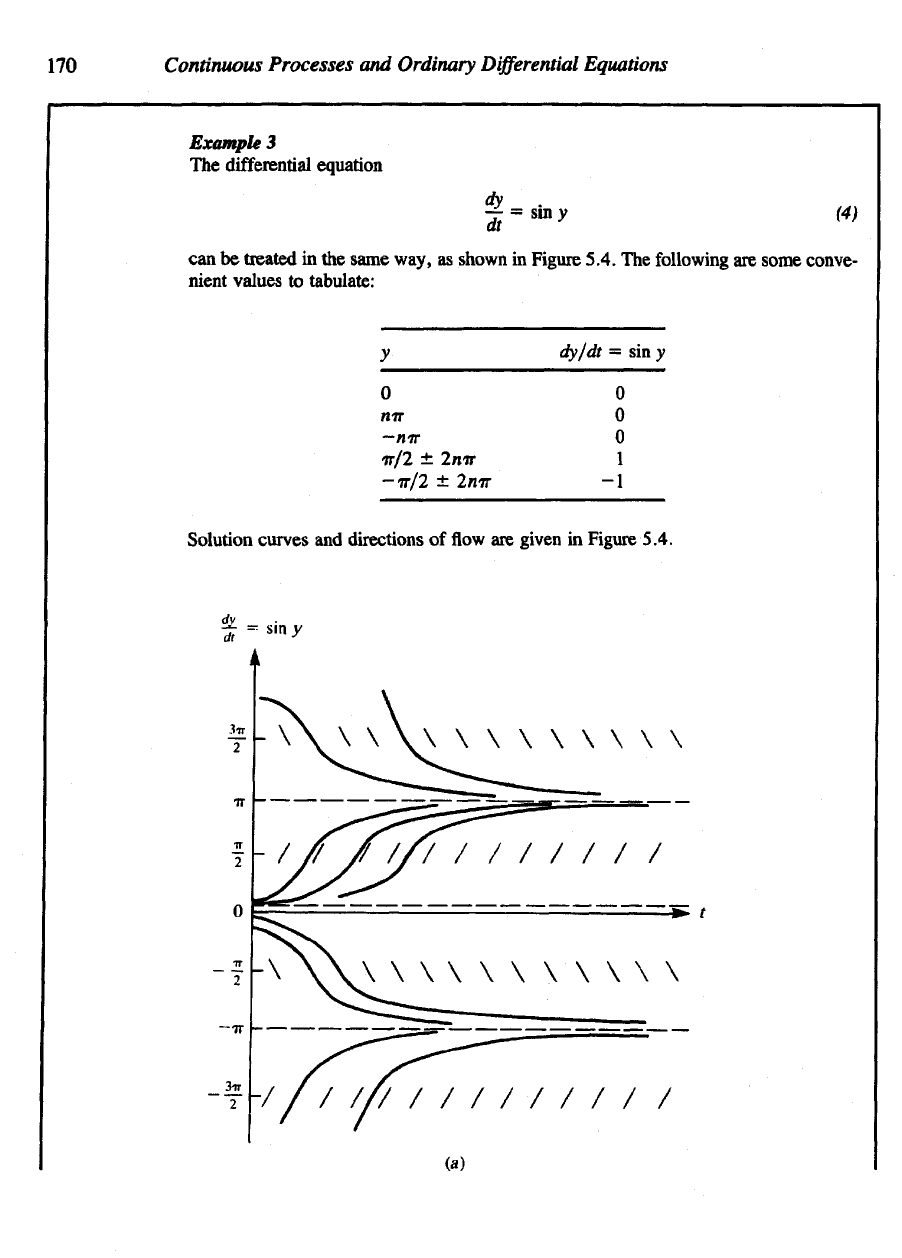
Example

3

The

differential

equation

can be

treated

in the

same way,

as

shown

in

Figure 5.4.

The

following

are

some conve-

nient values

to

tabulate:

Solution curves

and

directions

of flow are

given

in

Figure 5.4.

y

0

ntr

—nir

ir/2

±

2nir

-it/2

±

2nir

dy/dt

= sin y

0

1

-1

Phase-Plane

Methods

and

Qualitative

Solutions

171

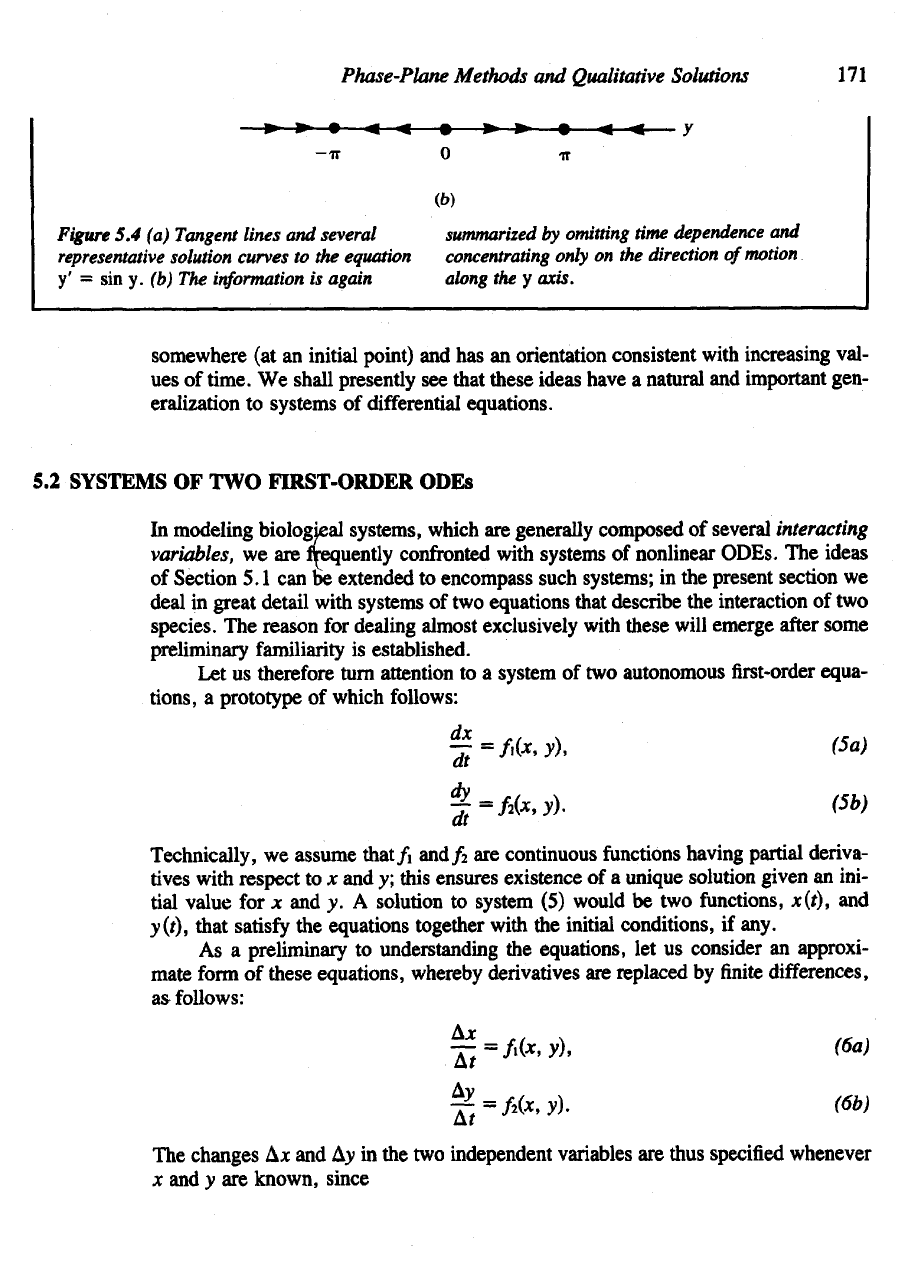
Figure

5.4 (a)

Tangent lines

and

several summarized

by

omitting

time

dependence

and

representative

solution curves

to the

equation concentrating

only

on the

direction

of

motion

y' = sin y. (b) The

information

is

again

along

the y

axis.

somewhere

(at an

initial point)

and has an

orientation consistent

with

increasing val-

ues

of

time.

We

shall presently

see

that these ideas have

a

natural

and

important gen-

eralization

to

systems

of

differential equations.

5.2

SYSTEMS

OF TWO

FIRST-ORDER ODEs

In

modeling

biological

systems, which

are

generally composed

of

several interacting

variables,

we are

frequently confronted with systems

of

nonlinear ODEs.

The

ideas

of

Section

5.1 can be

extended

to

encompass such systems;

in the

present section

we

deal

in

great detail with systems

of two

equations that describe

the

interaction

of two

species.

The

reason

for

dealing almost exclusively with these will emerge

after

some

preliminary familiarity

is

established.

Let us

therefore turn attention

to a

system

of two

autonomous

first-order

equa-

tions,

a

prototype

of

which follows:

Technically,

we

assume

that/i

and/2

are

continuous functions having partial deriva-

tives

with

respect

to x and y;

this ensures

existence

of a

unique solution given

an

ini-

tial value

for x and y. A

solution

to

system

(5)

would

be two

functions, x(t),

and

y

(t),

that satisfy

the

equations together with

the

initial conditions,

if

any.

As

a

preliminary

to

understanding

the

equations,

let us

consider

an

approxi-

mate

form

of

these equations, whereby derivatives

are

replaced

by finite

differences,

a&

follows:

The

changes

A* and Ay in the two

independent varizbles are thus specified whenever

x and y are

known, since

172

Continuous Processes

and

Ordinary

Differential

Equations

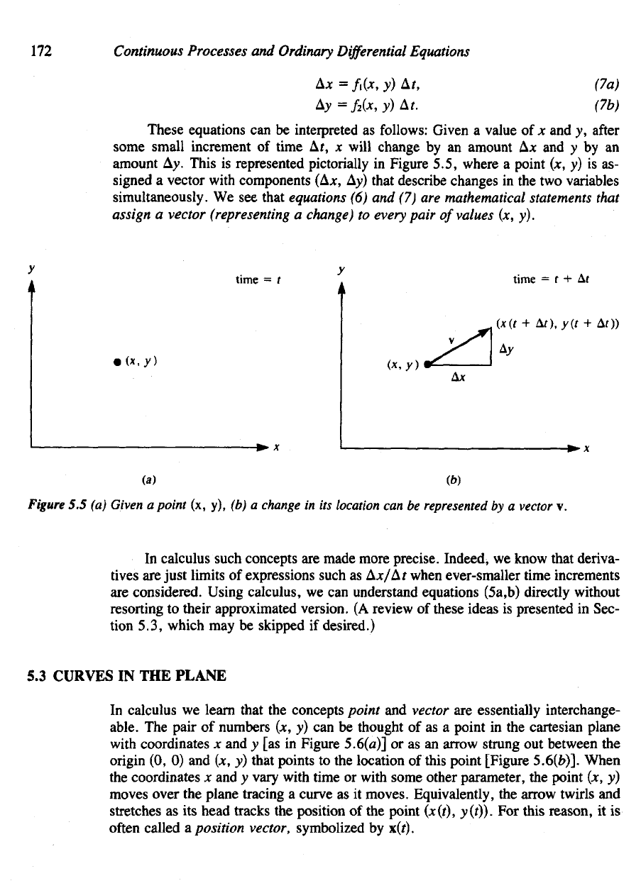
These equations

can be

interpreted

as

follows:

Given

a

value

of x and y,

after

some

small increment

of

time

Af, x

will change

by an

amount

AJC

and y by an

amount

Ay.

This

is

represented pictorially

in

Figure 5.5, where

a

point

(x, y) is as-

signed

a

vector

with

components (A*,

Ay)

that describe changes

in the two

variables

simultaneously.

We see

that equations

(6) and (7) are

mathematical statements that

assign

a

vector (representing

a

change)

to

every

pair

of

values

(x, y).

Figure

5.5 (a)

Given

a

point

(x, y), (b) a

change

in its

location

can be

represented

by a

vector

v.

In

calculus such concepts

are

made more

precise.

Indeed,

we

know that deriva-

tives

are

just limits

of

expressions such

as

A*/A/ when ever-smaller time increments

are

considered. Using calculus,

we can

understand equations (5a,b) directly without

resorting

to

their approximated version.

(A

review

of

these ideas

is

presented

in

Sec-

tion 5.3, which

may be

skipped

if

desired.)

5.3

CURVES

IN THE

PLANE

In

calculus

we

learn that

the

concepts point

and

vector

are

essentially interchange-

able.

The

pair

of

numbers (jc,

y) can be

thought

of as a

point

in the

cartesian plane

with

coordinates

x and y [as in

Figure

5.6(a)]

or as an

arrow strung

out

between

the

origin

(0, 0) and (x, y)

that

points

to the

location

of

this

point

[Figure

5.6(&)]. When

the

coordinates

x and y

vary with time

or

with some other parameter,

the

point

(x, y)

moves over

the

plane tracing

a

curve

as it

moves. Equivalently,

the

arrow twirls

and

stretches

as its

head

tracks

the

position

of the

point

(x(t),

y(t)).

For

this

reason,

it is

often

called

a.

position vector, symbolized

by

x(f).

Phase-Plane

Methods

and

Qualitative Solutions

173

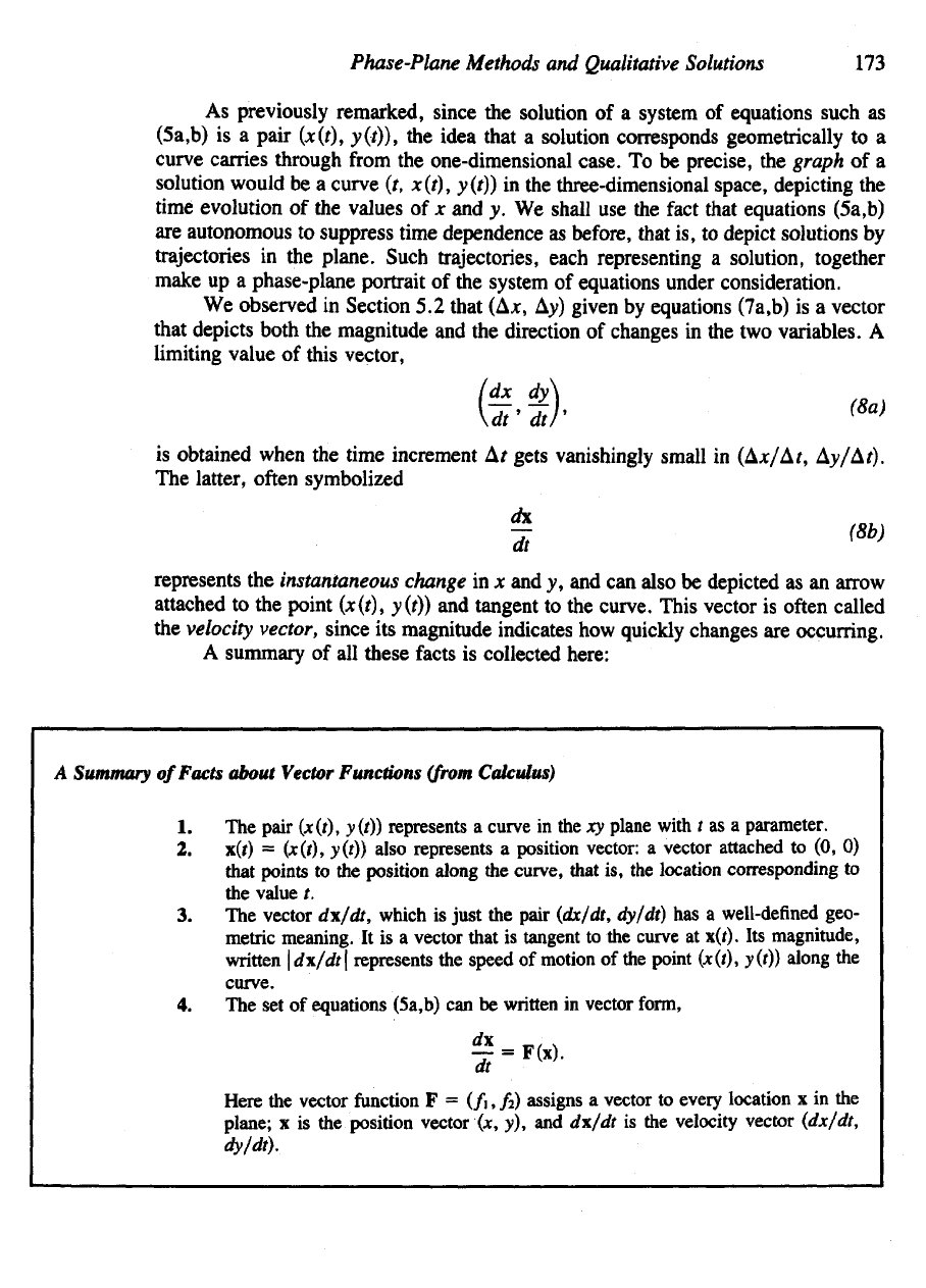
As

previously remarked, since

the

solution

of a

system

of

equations such

as

(5a,b)

is a

pair

(x(t),

y(/)),

the

idea that

a

solution corresponds geometrically

to a

curve

carries

through

from

the

one-dimensional case.

To be

precise,

the

graph

of a

solution would

be a

curve

(t,

x(t), y(t))

in the

three-dimensional space, depicting

the

time evolution

of the

values

of x and y. We

shall

use the

fact

that equations (5a,b)

are

autonomous

to

suppress time dependence

as

before, that

is, to

depict solutions

by

trajectories

in the

plane. Such trajectories, each representing

a

solution,

together

make

up a

phase-plane portrait

of the

system

of

equations under consideration.

We

observed

in

Section

5.2

that (A*,

Ay)

given

by

equations (7a,b)

is a

vector

that

depicts both

the

magnitude

and the

direction

of

changes

in the two

variables.

A

limiting

value

of

this vector,

is

obtained

when

the

time increment

Af

gets vanishingly small

in

(Ax/Ar,

Ay/Af).

The

latter, often symbolized

represents

the

instantaneous change

in x and y, and can

also

be

depicted

as an

arrow

attached

to the

point

(x(t),

y(f))

and

tangent

to the

curve. This vector

is

often

called

the

velocity

vector, since

its

magnitude indicates

how

quickly changes

are

occurring.

A

summary

of all

these

facts

is

collected

here:

A

Summary

of

Facts

about

Vector

Functions

(from

Calculus)

1. The

pair

(x(t),

y(t))

represents

a

curve

in the xy

plane

with

t as a

parameter.

2.

x(f)

=

(x(t),

y(t)) also

represents

a

position

vector:

a

vector

attached

to (0, 0)

that

points

to the

position along

the

curve,

that

is, the

location

corresponding

to

the

value

t.

3. The

vector

d\/dt,

which

is

just

the

pair

(dx/dt,

dy/dt)

has a

well-defined

geo-

metric

meaning.

It is a

vector

that

is

tangent

to the

curve

at

x(f).

Its

magnitude,

written

\d\fdt\

represents

the

speed

of

motion

of the

point

(x(t),

y(t))

along

the

curve.

4. The set of

equations (5a,b)

can be

written

in

vector

form,

Here

the

vector

function

F =

(f\,

/

2

)

assigns

a

vector

to

every

location

x in the

plane;

x is the

position vector

(x, y), and

d\/dt

is the

velocity

vector

(dx/dt,

dy/dt).

174

Continuous Processes

and

Ordinary

Differential

Equations

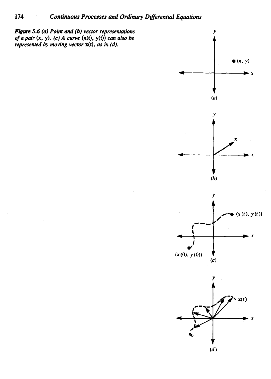
Figure

5.6 (a)

Point

and (b)

vector representations

of

a

pair

(x, y). (c) A

curve

(x(t),

y(t))

can

also

be

represented

by

moving vector

x(t),

as in

(d).

Phase-Plane

Methods

and

Qualitative

Solutions

175

5.4 THE

DIRECTION FIELD

From

c

that arise

in

calculus

we

surmise that solutions

to

ODEs, whether

in

one

dimension

or

higher, correspond

to

curves,

and

differential equations

are

"recipes"

for

tangent vectors

to

these curves. This insight will

now be

applied

to re-

constructing

a

qualitative picture

of

solutions

to a

system

of two

equations such

as

(5).

For

such autonomous systems each point

(x, y) in the

plane

is

assigned

a

unique

vector

(fi(x,

v),

f

2

(x,

y))

that does

not

change

with

time.

A

solution curve passing

through

(jc,

v)

must have these vectors

as its

tangents. Thus

a

collection

of

such vec-

tors

defines

a

direction

field,

which

can be

used

as a

visual guide

in

sketching

a

fam-

ily

of

solution curves, collectively

a

phase-plane portrait. Example

4

clarifies

how

this

is

done

in

practice.

After

tabulating arbitrarily many values

of (x, y) and the

corresponding values

of

f\(x,

y)

and/

2

(jc,

y), we are

ready

to

construct

the

direction

field. To

each point

(x,

y) we

attach

a

small

line

segment

in the

direction

of the

vector

(fi(x,

y),/2(x, y)).

Example

4

Let

and

let/iOc,

y) = xy —

y,/2(x,

y) = xy — x. In the

following

table

the

values

of/i

and

/2

are

listed

for

several values

of (x, y).

X

0

1

-1

0

1

-2

y

0

i

0

__

i

-i

MX,

y)

0

-i

0

i

0

2

3

h(x,

y)

0

-1

1

0

-2

4

Edelstein-Keshet L. Mathematical Models in Biology

Подождите немного. Документ загружается.