Edelstein-Keshet L. Mathematical Models in Biology

176

Continuous

Processes

and

Ordinary

Differential

Equations

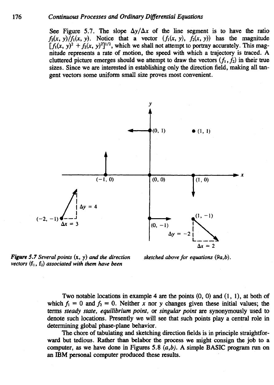
See

Figure 5.7.

The

slope Ay/A*

of the

line segment

is to

have

the

ratio

f

2

(x,

y)/f\(x,

v).

Notice that

a

vector

(fi(x,

v),

f

2

(x,

v)) has the

magnitude

[/i(*i

y)

2

+

/2(*>

y)

2

]

1/2

,

which

we

shall

not

attempt

to

portray accurately. This mag-

nitude represents

a

rate

of

motion,

the

speed

with

which

a

trajectory

is

traced.

A

cluttered picture emerges should

we

attempt

to

draw

the

vectors (/i,

fa) in

their true

sizes.

Since

we are

interested

in

establishing only

the

direction

field,

making

all

tan-

gent vectors some

uniform

small size proves most convenient.

Two

notable locations

in

example

4 are the

points

(0, 0) and (1, 1), at

both

of

which

/i = 0 and /

2

= 0.

Neither

x nor v

changes given these initial values;

the

terms

steady

state, equilibrium point,

or

singular point

are

synonymously used

to

denote such locations. Presently

we

will

see

that such points play

a

central

role

in

determining global phase-plane behavior.

The

chore

of

tabulating

and

sketching direction

fields is in

principle

straightfor-

ward

but

tedious. Rather than belabor

the

process

we

might consign

the job to a

computer,

as we

have done

in

Figures

5.8

(a,b).

A

simple BASIC program

run on

an

IBM

personal computer produced these results.

Figure

5.7

Several points

(x, y) and the

direction

vectors

(f

i, f

2

)

associated with them have been

sketched

above

for

equations (9a,b).

Figure

5.8 (a)

Computer-generated vector

field for

solution curves

for

example

4. The

directions

are

example

4. The

vectors

point

sway

from

the

points ascertained

by

noting whether vectors

point

into

or

to

which

they

are

attached.

For

example, along

the out

of

the

region

at the

boundary

of

the

square,

positive

x

axis,

they

point

down,

(b)

Hand-sketched

(Computer

plot

by

Yehoshua

Keshet.)

178

Continuous Processes

and

Ordinary

Differential

Equations

From

the

direction

field

thus

generated

one

gets

a

good general idea

of

solution

curves consistent with

the flow.Through

every point

in the

plane there

is a

curve

(by

existence

of a

solution)

and

only

one

curve

(by

uniqueness). Thus curves

may not in-

tersect

or

touch

each

other,

except

at the

steady states designated

by

heavy dots

in

Figures

5.7 and

5.8. Rules governing

the

possible pattern

of

curves will

be

outlined

in

a

subsequent section.

As a

word

of

caution, note that

a

phase-plane diagram

is not a

quantitatively

accurate graph.

In

practice, because only

a finite

number

of

tangent vectors

can be

drawn

in the

plane, there will always

be

some small error

in the

curve that

we in-

scribe. Such initially small mistakes could propagate

if

they result

in an

improper

choice

of

tangent vectors along

the

way.

For

this reason, solution curves drawn

in

this

way are

approximate. There

may be

cases where ambiguity arises close

to a

steady

state

and

where

it is

difficult

to

distinguish between

several

alternatives. Such

situations call

for a

more

rigorous

technique. Before turning

to

these matters,

we in-

vestigate

a

more systematic

way of

establishing

the

direction

field in a

computation-

ally

efficient

way.

5.5

NULLCLINES:

A

MORE SYSTEMATIC APPROACH

Rather

than arbitrarily plotting tabulated values,

we

prepare

the way by

noticing

what

happens

along

the

locus

of

points

for

which

one of the two

functions,

either

fi(x,

v)

or/

2

(jc,

y) is

zero.

We

observe that

1. If

fi(x,

y) = 0,

then dx/dt

= 0, so x

does

not

change. This means that

the

direction vector must

be

parallel

to the y

axis, since

its

AJC

component

is

zero.

2.

Similarly,

if

f

2

(x,

y) = 0,

then dy/dt

= 0, so y

does

not

change. Thus

the

direction vector

is

parallel

to the x

axis, since

its Ay

component

is

zero.

The

locus

of

points satisfying

one of

these

two

conditions

is

called

a

nullcline.

The x

nullcline

is the set of

points satisfying condition

1;

similarly,

the y

nullcline

is

the

set of

points satisfying condition

2.

Because

the

arrows

are

parallel

to the y and x

axis

respectively

on

these

loci,

it

proves

helpful

to

sketch these

as a first

step. Exam-

ple

5

illustrates

the

procedure.

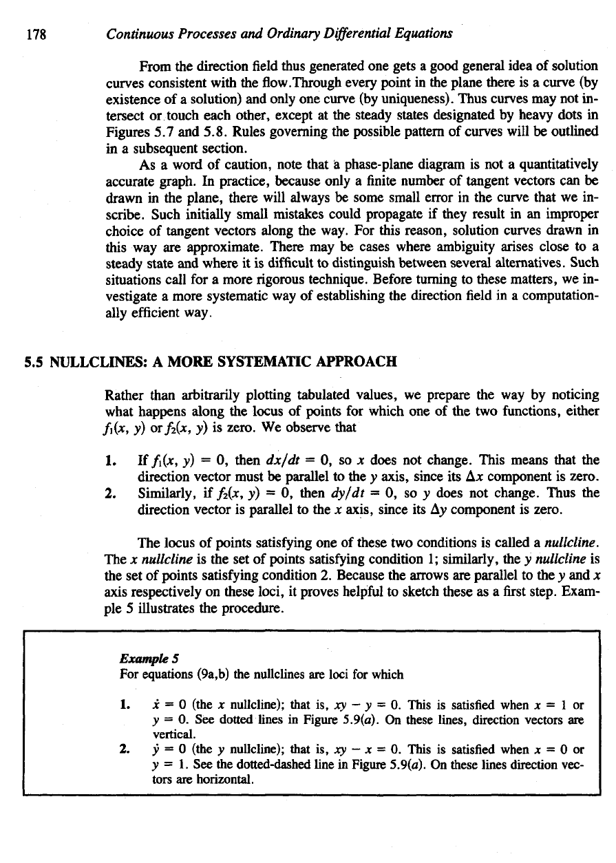
Example

5

For

equations (9a,b)

the

nullclines

are

loci

for

which

1. x = 0

(the

x

nullcline); that

is, xy — y = 0.

This

is

satisfied when

x = 1 or

y

= 0. See

dotted lines

in

Figure

5.9(a).

On

these lines, direction vectors

are

vertical.

2. y = 0

(the

y

nullcline); that

is, xy - x = 0.

This

is

satisfied when

x = 0 or

y

= 1. See the

dotted-dashed line

in

Figure 5.9(a).

On

these lines direction vec-

tors

are

horizontal.

Phase-Plane

Methods

and

Qualitative

Solutions

179

Figure

5.9

Nullclines

and flow

directions

for

example

5. (a)

Nullclines, which happen

to

be

straight lines here,

are

sketched

in the

xy-plane

and

assigned vertical

or

horizontal

line

segments

in

(b).

(c)

Directions

are

determined

by

tabulating several values

and

inscribing

arrowheads,

(d)

Neighboring

arrows

are

deduced

by

preserving

a

continuous flow.

Points

of

intersection

of

nullclines

satisfy

both

x = 0 and y = 0 and

thus

rep-

resent steady states.

To

identify

these

and

determine

the

directions

of flow,

several

guidelines

are

useful.

180

Continuous Processes

and

Ordinary

Differential

Equations

Rules

for

determining

steady

states

and

direction vectors

on

nullclines

1.

Steady states

are

located

at

intersections

of an *

nullcline

with

a y

nullcline.

2. At

steady states there

is no

change

in

either

x or y

values; that

is, the

vectors

have zero length.

3.

Direction vectors must vary continuously

from one

point

to the

nullclines. Thus

a

change

in the

orientation (for example,

from

pointing

up to

pointing down)

can

take place only

at

steady states.

We

note

that

(0, 0) and (1, 1) are the

only

two

steady states

in

example

5. It is im-

portant

to

avoid confusing these with other intersections,

for

example (1,0)

and

(0, 1), for

which only

one of the two

nullcline conditions

is

satisfied. Generally

it is

a

good idea

to

distinguish between

the x and y

nullclines

by

using

different

symbols

or

colors

for

each type.

It

should

be

remarked that

in

affixing

orientations

to the

arrows along null-

clines

we can

economize

on

algebra

by

being aware

of

certain geometric properties.

For

instance,

in

example

5 we

observe

the

following

patterns

of

signs:

X

0

1

0

+ , > 1

1

0

—

y

i

-

+

i

+,

> i

+

0

/.(*,

y)

+

0

+

0

-

0

/a(*.

y)

0

-

0

+

0

+

It

is

evident that

on

opposite sides

of a

steady-state point (along

a

given null-

cline)

the

orientation

of

arrows

is

reversed. This

is a

property shared

by

most sys-

tems

of

equations with

the

exception

of

certain singular cases.

(We

shall

be

able

to

distinguish

these exceptions

by

calculating

the

Jacobian

J and

evaluating

it at the

steady state

in

question.

If det J

=£

0, the

property

of

arrow reversal holds.)

In

most

cases

where

we

encounter

det J ^ 0, it

suffices

to

determine

the

direction vectors

at

one or two

select places

and

deduce

the

rest

by

preserving continuity

and

switching

orientation

as a

steady state

is

crossed.

Thus

the

arrow-nullcline method

can

reveal

a

fairly

complete picture with relatively

little

calculation (see example

6).

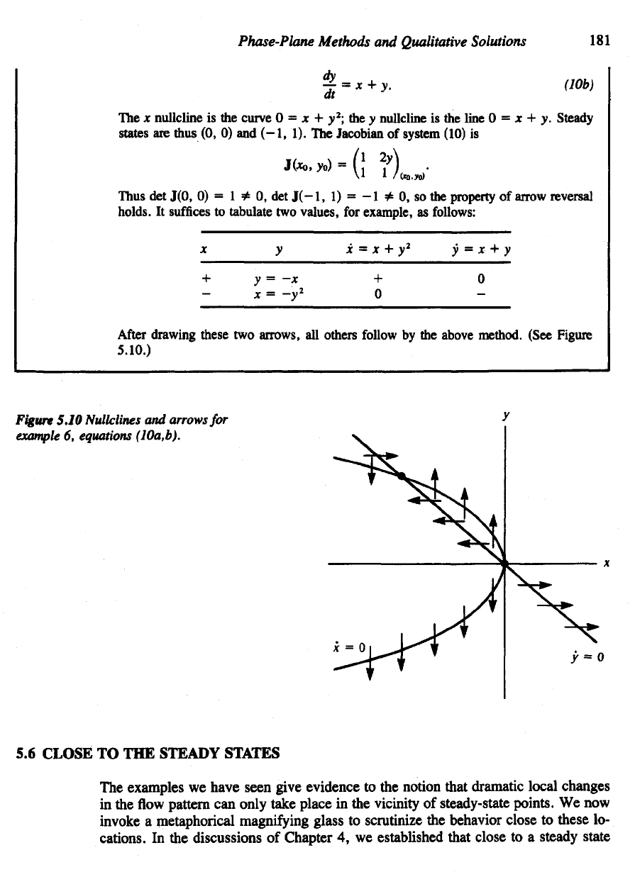
Example

6

Consider

the

equations

Phase-Plane

Methods

and

Qualitative

Solutions

181

The

x

nullcline

is the

curve

0 = x + y

2

; the y

nullcline

is the

line

0 = x + y.

Steady

states

are

thus

(0, 0) and

(-1,

1). The

Jacobian

of

system

(10)

is

Thus

det

J(0,

0) = 1 * 0, det

J(-l,

1) = -1 * 0, so the

property

of

arrow reversal

holds.

It

suffices

to

tabulate

two

values,

for

example,

as

follows:

After

drawing these

two

arrows,

all

others follow

by the

above method.

(See

Figure

5.10.)

Figure

5.10

Nullclines

and

arrows

for

example

6,

equations (10a,b).

5.6

CLOSE

TO THE

STEADY STATES

The

examples

we

have seen give evidence

to the

notion that dramatic local changes

in

the flow

pattern

can

only take place

in the

vicinity

of

steady-state points.

We now

invoke

a

metaphorical

magnifying

glass

to

scrutinize

the

behavior close

to

these

lo-

cations.

In the

discussions

of

Chapter

4, we

established that close

to a

steady state

X

+

-

y

y=-x

x=-y*

x

= x + y

2

+

0

y

= x + y

0

-

182

Continuous Processes

and

Ordinary

Differential

Equations

(XQ,

yo)

[defined by/i(x

0

,

yo) =

/2(*

0

,

yo) = 0] the

nonlinear system

(5)

behaves very

nearlv like

a

linear one.

where a

tj

, related

to

partial derivatives of/i

and/

2

,

make

up the

coefficient

of the Ja-

cobian matrix J(J

0

,

yo) as

follows:

This result

is

important,

as it

reduces

the

problem

to one we

understand well.

It

remains

to

interpret

the

phase-plane equivalents

of

solutions

to

systems

of

linear

ODEs (described

in

Chapter

4).

This will give

us the

local picture

of the flow

pattern

about

the

steady states.

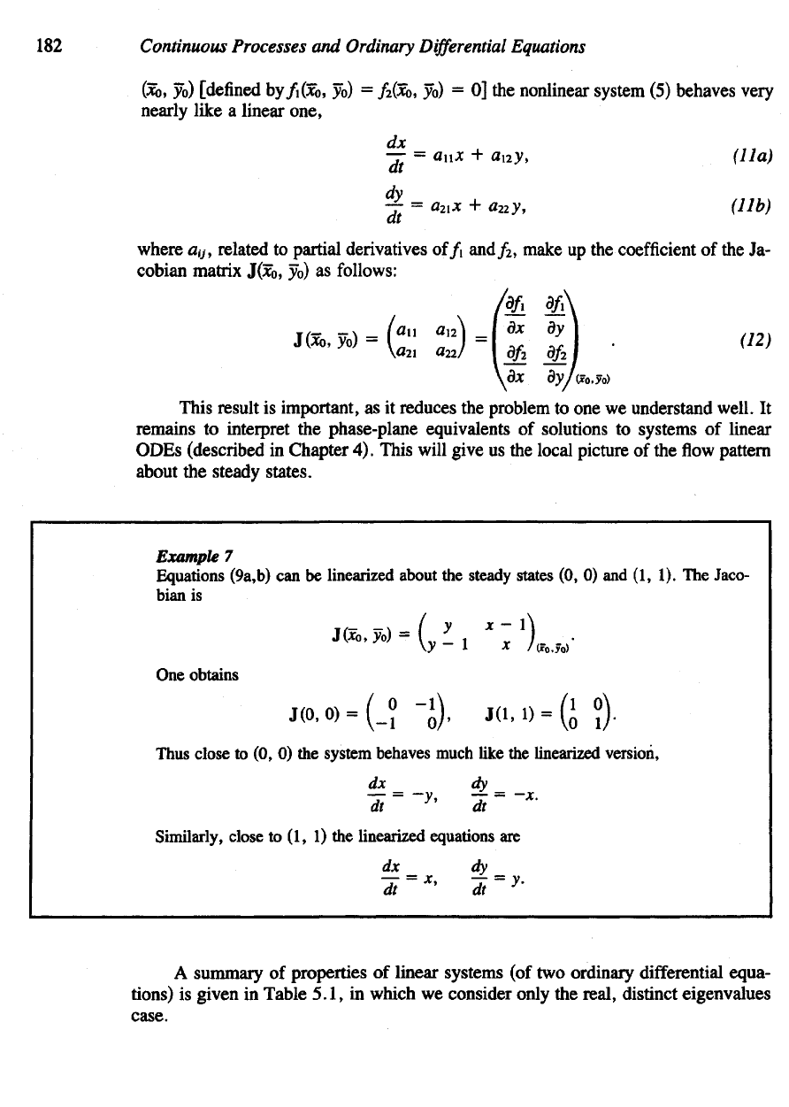
Example

7

Equations (9a,b)

can be

linearized about

the

steady states

(0, 0) and (1, 1). The

Jaco-

bian

is

One

obtains

Thus

close

to (0, 0) the

system behaves much like

the

linearized

version

Similarly,

close

to (1, 1) the

linearized

equations

are

A

summary

of

properties

of

linear

systems

(of two

ordinary differential equa-

tions)

is

given

in

Table 5.1,

in

which

we

consider only

the

real, distinct eigenvalues

case.

Table

5.1

Linear

Systems

of two

ODEs

Equations

Significant

quantities

Characteristic equation

Eigenvalues

Identities

Eigenvectors

Solutions

Full

algebraic notation

jB

= OH +

0

2

2,

7 — On 0

2

2 ~

012021,

S

=

j8

2

- 4y

A

2

-

j8A

+. y = 0

A,

+ A

2

= j8,

jc

=

Cifli

2

e

A

«'

+

c

2

a

12

e

A2

',

y

=

d,e

A

i'

+ rf

2

c

A

2',

where

d\ -

CI(AI

- flu), d

2

=

c

2

(A

2

-

an).

Equivalent

Vector-Matrix Notation

Tr

A,

det

A,

disc

A

det

(A

- Al) = 0

A,

+ A

2

= Tr A,

A,A

2

= det A

YI

, v

2

such that

(A -

AI)v,

= 0

X

=

CiVi6

A

l'

+

C

2

V

2

C

A

2'.

£81

184

Continuous Processes

and

Ordinary

Differential

Equations

5.7

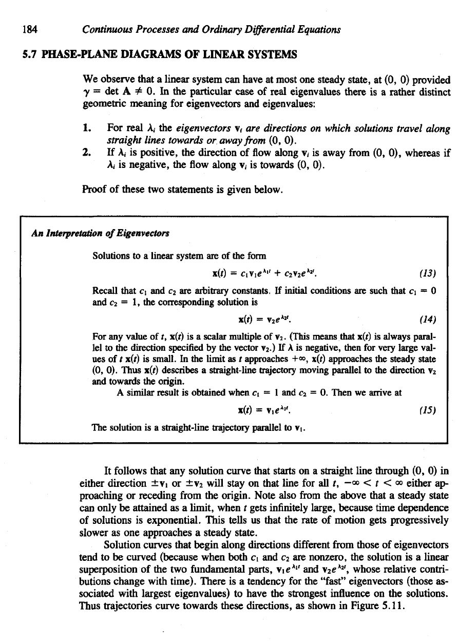
PHASE-PLANE DIAGRAMS

OF

LINEAR SYSTEMS

We

observe

that

a

linear system

can

have

at

most

one

steady state,

at (0, 0)

provided

y = det A

¥=

0. In the

particular

case

of

real eigenvalues there

is a

rather distinct

geometric meaning

for

eigenvectors

and

eigenvalues:

1. For

real

A, the

eigenvectors

v, are

directions

on

which solutions travel

along

straight

lines

towards

or

away

from

(0, 0).

2. If A, is

positive,

the

direction

of flow

along

v, is

away

from

(0, 0),

whereas

if

A,

is

negative,

the flow

along

v, is

towards

(0, 0).

Proof

of

these

two

statements

is

given below.

An

Interpretation

of

Eigenvectors

Solutions

to a

linear system

are of the

form

It

follows that

any

solution curve that starts

on a

straight line through

(0, 0) in

either direction

±Vi or ±v

2

will stay

on

that line

for all t, —« < t < «

either

ap-

proaching

or

receding

from

the

origin. Note also

from the

above that

a

steady state

can

only

be

attained

as a

limit, when

t

gets

infinitely

large, because time dependence

of

solutions

is

exponential. This tells

us

that

the

rate

of

motion gets progressively

slower

as one

approaches

a

steady state.

Solution curves that begin along directions

different

from

those

of

eigenvectors

tend

to be

curved (because when both

c\ and c

2

are

nonzero,

the

solution

is a

linear

superposition

of the two

fundamental parts,

VI£

AI

'

and

v

2

e

A2

', whose relative contri-

butions

change with time). There

is a

tendency

for the

"fast" eigenvectors (those

as-

sociated with largest eigenvalues)

to

have

the

strongest influence

on the

solutions.

Thus

trajectories curve towards these directions,

as

shown

in

Figure 5.11.

Recall that

c\ and c

2

are

arbitrary constants.

If

initial conditions

are

such that

c\ = 0

and

c-i

= 1, the

corresponding solution

is

For any

value

of /,

x(f)

is a

scalar multiple

of v

2

.

(This means that \(t)

is

always paral-

lel to the

direction specified

by the

vector v

2

.)

If A is

negative, then

for

very large val-

ues

of t

x(i)

is

small.

In the

limit

as t

approaches +°°, x(t) approaches

the

steady state

(0, 0).

Thus x(r)

describes

a

straight-line trajectory moving parallel

to the

direction

v

2

and

towards

the

origin.

A

Edelstein-Keshet L. Mathematical Models in Biology

Подождите немного. Документ загружается.