Fowler A. Mathematical Geoscience

Подождите немного. Документ загружается.

280 5 Dunes

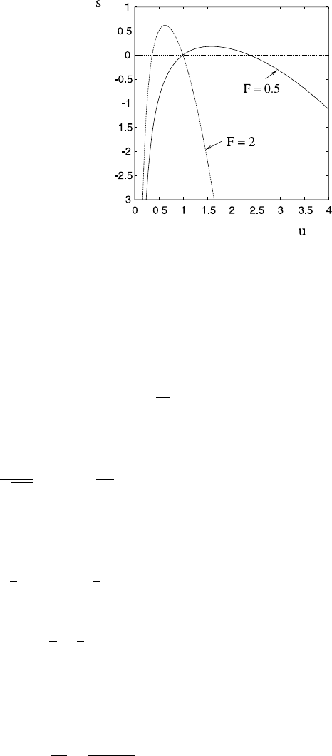
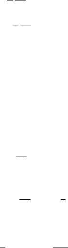
Fig. 5.10 s(u) as given by

(5.36) for two typical cases of

rapid and tranquil ﬂow

and we choose h

by balancing terms as follows: uh ∼ Q

, gS ∼fu

/h; here

is the (prescribed) volume ﬂow per unit width. We choose q

as the size of the

bedload transport equation in (5.5).

With these scales, the dimensionless equations corresponding to (5.31)are

=0,

εh

+(uh)

=0,

(εu

+uu

) =−η

+δ



1 −



h =η −s,

(5.33)

where the parameters are

F =

√

,ε=

,δ=S. (5.34)

If we now suppose ε  1 and δ  1, both of them realistic assumptions, then we

have approximately

uh = 1,

+η =

+1,

(5.35)

supposing that u, h →1 at large distances. Eliminating h and η,wehave

s =1 −



1 −u



, (5.36)

whose form is shown in Fig. 5.10. In particular, s



(1) = (1 −F

), so the basic state

u =1 corresponds to the left hand or right hand root of s(u) depending on whether

the Froude number F<1orF>1.

We also have

dη

−h

, (5.37)

5.4 St. Venant Type Models 281

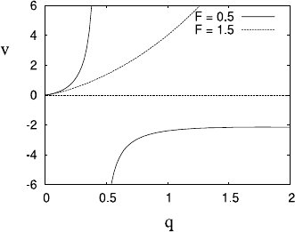
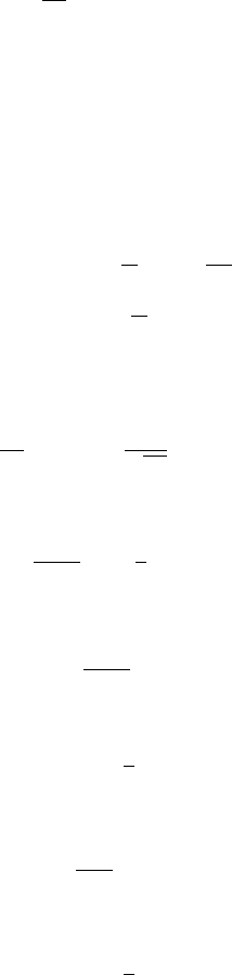
Fig. 5.11 The wave speed

v(q) =3q

4/3

/(1 −F

q) for

the tranquil and rapid cases

F =0.5andF =1.5

so that small perturbations to h =1 are out of phase (dunes) if F<1 and in phase

(anti-dunes) if F>1. If we take the dimensionless bedload transport as q ≈τ

3/2

(the dimensionless basal stress having been scaled with fρ

), so that u =q

1/3

then we see from (5.36) that s = s(q), and s(q) has the same shape as s(u),asshown

in Fig. 5.10.

The whole model reduces to the single ﬁrst order equation



(q)q

=0. (5.38)

Disturbances to the uniform state q = 1 will propagate at speed v(q) = 1/s



(q),

where v isshowninFig.5.11.ForF<1, v(1)>0 and v



(1)>0, thus waves in q

(and thus s) propagate downstream and form forward-facing shocks; this is nicely

consistent with dunes. For F>1, v<0 and v



(1) is positive if F<2, negative if

F>2 (see Question 5.4). Backward-facing shocks form, these are elevations in s if



> 0.

Unfortunately, the hyperbolic equation does not admit instability. It is straight-

forward to insert a lag as before, by writing q(x,t) =q[s(x −δ,t)], or equivalently

s(x,t) =s[q(x +δ,t)]. Perturbation of

=0,

q =q



s(x −δ,t)



(5.39)

via

s =¯se

ikx+σt

,q=1 +¯qe

ikx+σt

, (5.40)

leads to

σ ¯s +ik ¯q =0,

¯q =q



−ikδ

¯s,

(5.41)

and thus

σ =kq



[−sin kδ −i coskδ]. (5.42)

This requires sinkδ < 0 for instability if q



(s) > 0 (F < 1) and sinkδ > 0ifq



(s) <

0 (F > 1). The long wavelength limit of (5.26) in which kh →0 is precisely (5.42),

bearing in mind that (5.26) is dimensional and that q



=dq/du there, whereas q



dq/ds in (5.42).

282 5 Dunes

5.5 A Suspended Sediment Model

The shortcoming of both the potential model and the St. Venant/Exner model is the

lack of a genuine instability mechanism. We now show that the inclusion of sus-

pended load can produce instability. Ideally, we would hope to predict anti-dunes,

since dunes certainly do not require suspended sediment transport. A St. Venant

model including both bedload and suspended sediment transport is

+(uh)

=0,

+uu

=g(S −η

) −

∂

∂t

(hc) +

∂

∂x

(hcu) =ρ

−v

(1 −n)

∂s

∂t

∂q

∂x

=−(v

−v

(5.43)

where c is the column average concentration (mass per unit volume) of suspended

sediment (written as ¯c earlier). The distinction between suspended sediment trans-

port and bedload lies in the source terms due to erosion and deposition, v

and

, and it is these which may enable instability to occur. We have η −s = h, and

we suppose q

(τ ), τ =fρ

, whence q = q(u). Additionally (see (5.7) and

(5.10)), we write

E, ρ

cD, (5.44)

and expect that E = E(u) and D = D(u), with E



> 0, D



< 0; typically E<1,

D>1.

We scale (5.43) as before in (5.32), except that we choose the time scale t

downstream length scale x

, and concentration scale c

via

=ρ

(1 −n)h

, (5.45)

where we write

E =E

∗

(u/u

), D =D

∗

(u/u

), (5.46)

and choose E

and D

so that E

∗

and D

∗

are O(1), and so that these are consistent

with typical observed suspended loads of 10 g l

−1

. With this choice of scales, we

obtain the dimensionless set of equations

η −s =h,

εh

+(uh)

=0,

(εu

+uu

) =δ



1 −



−η

h(εc

+uc

) =E

∗

−cD

∗

+βq

=−(E

∗

−cD

∗

(5.47)

5.5 A Suspended Sediment Model 283

where the parameters ε, F, δ and β are now given by

ε =

(1 −n)D

(1 −n)

,δ=

F =

(gh

)

1/2

,β=

(5.48)

Here q

is the scale for q

rather than q = q

/(1 − n). The Froude number is

the same as before, but the parameters ε and δ are different: ε is a measure of

the suspended sediment density relative to the bed density, and is always small;

δ is the ratio of the (small) bed slope to the ratio of settling velocity to stream

velocity. For more rapidly ﬂowing streams, we might expect δ ∼1. However, if we

suppose that wavelengths of anti-dunes are comparable to the depth (so x

∼ h

then (5.45) implies δ ∼S 1. Thus δ ∼1 implies x

∼h

/S h

. The parameter

β is a direct measure of the ratio of bedload (ρ

) to suspended load (c

).For

β 1, we would revert to our preceding bedload model and its scaling, and neglect

the suspended load. If we adopt the Meyer-Peter/Müller relation in (5.5) and (5.6),

then (noting that fu

=gSh

)

Kρ

ρ

(ghS)

3/2

, (5.49)

and we can write

β =



Kρ

(1 −n)ρ



3/2

εF

; (5.50)

both small or large values are possible.

To analyse (5.47), we ignore bedload (put β =0) and take ε →0. Then

η =h +s, uh =1, (5.51)

so that

∗

(u) −cD

∗

(u) =−s

∂

∂x





=δ



1 −u



(5.52)

If, in addition, δ  1, then, taking s =0 when h =1,

s =s(u) =



1 −u



+1 −

, (5.53)

and the entire suspended load model is



(u)

∂u

∂t

=cD

∗

(u) −E

∗

(u) =−

∂c

∂x

. (5.54)

The function s(u) is the same as we derived before in (5.36) and shown in

Fig. 5.10. We can in fact write (5.54) as a single equation for u, by eliminating c;

this gives

c =

∗

(u)

∗

(u)



(u)

∗

(u)

∂u

∂t



(u)

∂u

∂t

∂

∂x



∗

(u)

∗

(u)



(u)

∗

(u)

∂u

∂t



=0,

(5.55)

284 5 Dunes

and the equation for u (or the pair for u, c) is of hyperbolic type. Note that natural

initial boundary conditions for (5.54) are to prescribe u at t = 0, x>0, and c at

x =0, t>0.

Let us examine the stability of the steady state u =1, c =1. We put

u =1 +Re



ikx+σt



,c=1 +Re



ikx+σt



, (5.56)

and linearise, to obtain (noting E

∗

(1) =D

∗

(1) =1)

ikC =



∗

(1) −D

∗

(1)



U −C =−σs



(1), (5.57)

and thus

σ =



∗

(1) −D

∗

(1)



(1)



−k

−ik

1 +k



. (5.58)

If we suppose E

∗

> 0, D

∗

< 0 as previously suggested, then this model im-

plies instability (Re σ>0) for s



(1)<0, i.e. F>1, and that the wave speed is

−Im(σ )/k < 0; thus this theory predicts upstream-migrating anti-dunes.

Two features suggest that the model is not well-posed if F>1. The ﬁrst is the

instability of arbitrarily small wavelength perturbations; the second is that the un-

stable waves propagate upstream, although the natural boundary condition for c is

prescribed at x =0.

Numerical solutions of (5.54) are consistent with these observations. In solving

the nonlinear model (5.54)in0<x<∞, we note that



∞

s(u)dx =−[c]

∞

, (5.59)

which simply represents the net erosion of the bed downwards if the sediment ﬂux

at inﬁnity is greater than at zero. It thus makes sense to ﬁx the initial boundary

conditions so that

c =1onx =0,

u →1asx →∞,t=0.

(5.60)

For F<1, numerical solutions are smooth and approach the stable solution

u =c =1. However, the solutions are numerically unstable for F>1, and u rapidly

blows up, causing breakdown of the solution.

Some further insight into this is gained by consideration of the solution at x =0.

If c =c

(t) on x = 0 and u = u

(x) on t =0, then we can obtain u on x = 0 from

(5.55), by solving the ordinary differential equation

∂u

∂t

∗

(u)



(u)

∗

(u)



(u)

(t) (5.61)

with u =u

(0) at t =0. If we suppose that c =1atx =0, then it is easy to show that

if F<1 and u(0, 0)<1/F

2/3

, then u(0,t)→ 1ast →∞. If on the other hand,

F>1 and u(0, 0)<1, then u(0,t)→1/F

2/3

in ﬁnite time, and the solution breaks

down as ∂u/∂t →∞;ifu(0, 0)>1, then u(0,t)→∞, again in ﬁnite time if, for

example, E

∗

∝u

. More generally, breakdown of the solution when F>1 occurs in

one of these ways at some positive value of x. Thus this suspended sediment model

shares the same weakness of the phase shift model in not appearing to provide a

well-posed nonlinear model.

5.6 Eddy Viscosity Model 285

5.6 Eddy Viscosity Model

The relative failure of the models above to explain dune and anti-dune formation

led to the consideration of a full ﬂuid ﬂow model, in which, rather than suppos-

ing that the ﬂow is shear free and that viscous effects were conﬁned to a turbulent

boundary layer, rotational effects were considered, and a model of turbulent shear

ﬂow incorporating an eddy viscosity, together with the Exner equation for bedload

transport, was adopted. This allows for a linear stability analysis of the uniform ﬂow

over a ﬂat bed via the solution of a suitable Orr–Sommerfeld equation. We shall in

fact proceed in somewhat more generality. As an observation, fully-formed dunes

have relatively small height to length ratios, and thus the ﬂuid ﬂow over them can

be approximately linearised. Although we use a linear approximation to derive the

stress at the bed, we may retain the nonlinear Exner equation for example. In this

way we may derive a nonlinear evolution equation for bed elevation.

5.6.1 Orr–Sommerfeld Equation

Suppose, therefore, that we have two-dimensional turbulent ﬂow down a slope of

gradient S, governed by the Reynolds equations

+uu

+wu

=−

∂p

∂x

+ν

∇

u +gS,

+uw

+ww

=−

∂p

∂z

+ν

∇

w −g



1 −S



1/2

=0,

(5.62)

where (u, w) are the velocity components and ν

is an eddy viscosity associated

with the Reynolds stress terms, such as prescribed in (B.9). In the second equation,

we can take g(1 −S

)

1/2

≈g since S is small.

We consider perturbations to a basic shear ﬂow u(z) in s<z<ηwhich satisﬁes

(5.62) with ν

taken as constant. (Later, we will study a more realistic eddy viscosity

model.) It is convenient ﬁrst of all to non-dimensionalise the Eqs. (5.62). In the basic

uniform state, with s =0 and η =

h, the shear ﬂow satisﬁes

∂u

∂z

=gS(

h −z), (5.63)

whence

u =



hz −



, (5.64)

and the column mean ﬂow is

¯u =



udz=

3ν

. (5.65)

286 5 Dunes

Taking ν

=ε

¯u

h, we ﬁnd that the basal shear stress is

τ =ρ

∂u

∂z



=fρ

¯u

, (5.66)

where f = 3ε

. This gives the relationship between the empirical f and the semi-

analytic ε

. If the bed and hence the ﬂow is perturbed, we would only retain constant

if the volume ﬂux per unit width is the same; this we therefore assume.

We now non-dimensionalise the variables by writing

(u, w) ∼¯u, (x, z) ∼

h, t ∼

h/ ¯u, p −ρg(

h −z) ∼ρ

¯u

. (5.67)

The dimensionless equations are

+uu

+wu

=−p

∇

u +

+uw

+ww

=−p

∇

=0,

(5.68)

and the parameters are a turbulent Reynolds number and the Froude number:

R =

¯u

,F=

¯u



. (5.69)

The dimensionless basic velocity proﬁle is then

u =

¯u



z −



, (5.70)

and the dimensionless mean velocity is, by deﬁnition of ¯u,

1 =

3ν

¯u

. (5.71)

Since

=ε

¯u

h =

f ¯u

h, (5.72)

this requires

¯u =





1/2

. (5.73)

In particular, the dimensionless basic velocity proﬁle is

u =U(z)=3



z −



. (5.74)

We now suppose that s and η are perturbed by small amounts; we may thus

linearise (5.68). We put

(u, w) =



U(z)+ψ

, −ψ



, (5.75)

5.6 Eddy Viscosity Model 287

whence it follows for small ψ that ψ satisﬁes the steady state Orr–Sommerfeld

equation

U∇

−U



−1

∇

ψ, (5.76)

where we assume stationary solutions in view of the anticipated fact that s evolves

on a slower time scale.

The condition of zero pressure at z =η is linearised to be

η =1 +F



z=1

. (5.77)

If F

is small, then we may take η to be constant, and we do so as we are primarily

interested in dunes. However, the dimensionless pressure p is only determined up

to addition of an arbitrary constant, which implies that the value of the constant η

is unconstrained. This represents the vertical translation invariance of the system. If

a uniform perturbation to s is made, then the response of the (uniform) stream is to

raise the surface by the same amount. We can remove the ambiguity by prescribing

η =1, with the implication that the mean value of s is required to be zero.

The other boundary conditions on z = s and z = 1 are no slip at the base, no

shear stress at the top, and the perturbed volume ﬂux is zero. These imply

ψ =0,ψ

=0onz =1,



U(z)dz+ψ =0,U+ψ

=0onz =s.

(5.78)

Linearisation of this second pair about z =0gives

ψ =0,ψ

=−U



s on z =0, (5.79)

where U



(0). Our aim is now to solve (5.76) with (5.78) and (5.79) to calculate

the perturbed shear stress. The dimensional basal shear stress is then

τ =ρ

¯u



1 +s







, (5.80)

and since f =3ε

=ε



, we may write this as

τ =fρ

¯u



1 +







. (5.81)

The problem to solve for ψ is linear and inhomogeneous, and so we suppose that

s =



∞

−∞

ˆs(k)e

ikx

dk, ψ =



∞

−∞

ψ(k)e

ikx

dk. (5.82)

(Note that ˆs will evolve slowly in time.) For each wave number k, we obtain







−k



−U







−2k





, (5.83)

with boundary conditions

ψ =



=0onz =1,

ψ =0,



=−U



ˆs on z =0,

(5.84)

288 5 Dunes

and thus we ﬁnally deﬁne

ψ =−U



ˆsΨ (z, k), (5.85)

where Ψ satisﬁes the canonical problem







−k



−U







−2k





Ψ =Ψ



=0onz =1,

Ψ =0,Ψ



=1onz =0.

(5.86)

In terms of Ψ , the basal (dimensional) shear stress is

τ =fρ

¯u



1 −s −



∞

−∞

ikx

ˆs(k)Ψ



(0,k)dk



. (5.87)

Using the convolution theorem, this is

τ =fρ

¯u



1 −s +



∞

−∞

K(x −ξ)s



(ξ) dξ



, (5.88)

where s



=∂s/∂x, and

K(x) =−

2π



∞

−∞



(0,k)

ikx

dk. (5.89)

Depending on K, we can see how τ may depend on displaced values of s. The form

of (5.88) illustrates our previous discussion of the vertical translation invariance of

the system. For a possible uniform perturbation s = constant, we would obtain a

modiﬁcation to the basic friction law, τ =fρ

¯u

. This is excluded by enforcing the

condition that s has zero mean in x,

lim

L→∞



−L

s(x)dx =0, (5.90)

which corresponds (for a periodic bed) to prescribing

ˆs(0) =0. (5.91)

To determine K, we need to know the solution of (5.86) for all k. In general,

the problem requires numerical solution. However, note that R =1/ε

, and is rea-

sonably large (for a value f = 0.005, R =3/f =600). This suggests that a useful

means of solving (5.86) may be asymptotically, in the limit of large R. The fact that

we can obtain analytic expressions for Ψ



(0,k) means this is useful even when R

is not dramatically large, as here.

The solution of the Orr–Sommerfeld equation at large R has a long pedigree, and

it is a complicated but mathematically interesting problem. We devote Appendix C

to ﬁnding the solution. We ﬁnd there that, for k>0,



(0,k)≈−3(ikRU



)

1/3

Ai(0) +O(1), (5.92)

where Ai is the Airy function. For k<0, Ψ



(0,k)= Ψ



(0, −k), and this leads to



(0,k)

≈



−ce

−iπ/3

|k|

−2/3

,k>0,

−ce

iπ/3

|k|

−2/3

,k<0,

(5.93)

5.6 Eddy Viscosity Model 289

where

c =3(RU



)

1/3

Ai(0), (5.94)

and c ≈1.54R

1/3

for U



=3, as Ai(0) =

2/3

(

)

≈0.355. From (5.89), we ﬁnd

K(x) =



∞

cos



kx −



2/3

. (5.95)

Evaluating the integral,

we obtain the simple formula

K(x) =

1/3

,x>0,

K(x) =0,x<0,

(5.96)

where

μ =

2/3

1/3









≈1.13R

1/3

. (5.97)

For stability purposes, note that

K =



∞

−∞

K(k)e

ikx

dk, (5.98)

where

K =−



(0,k)

2πik

c exp



−

iπ

sgnk



2π|k|

2/3

. (5.99)

5.6.2 Orr–Sommerfeld–Exner Model

We now reconsider (5.33), which we can write in the form

=0,

εh

+(uh)

=0,

(εu

+uu

) =−η

+δ



1 −



h =η −s.

(5.100)

Here τ is the local basal stress, scaled with fρ

. We suppose q = q(τ), so that

the Exner equation is

∂s

∂t



(τ )

∂τ

∂x

=0. (5.101)

How do we do that? The blunt approach is to consult Gradshteyn and Ryzhik (1980), where the

relevant formulae are on page 420 and 421 (items 4 and 9 of Sect. 3.761). The quicker way, using

complex analysis, is to evaluate



∞

ν−1

iθ

dθ (after a simple rescaling of k, k|x|=θ )byrotating

the contour by π/2 and using Jordan’s lemma. Thus



∞

ν−1

iθ

dθ =(ν)e

iπν/2