Freiling G., Yurko V. Lectures on Differential Equations of Mathematical Physics: A First Course

Подождите немного. Документ загружается.

232 G.

Freiling and V. Yurko

3. u

= a

, u(0,t) = A sin ωt, u(x,0) = 0, u

(x,0) = 0.

6.2.8. A semi-inﬁnite homogeneous string ( x ≥ 0 ) with the ﬁxed end-point x = 0 is

perturbed by the initial displacement

u(x,0) =











0, 0 ≤x ≤e,

−sin

πx

, e ≤x ≤ 2e,

0, 2e ≤x < ∞.

Find

the

form of the string at

t =

pro

vided

that the initial velocity is equal to zero, i.e. u

(x,0) = 0.

6.2.9. A homogeneous string of length l ( 0 ≤ x ≤ l ) is ﬁxed at the ends x = 0 and

x = l. At initial time t = 0 the string is deviated at the point x = l/3 to the distance h

from the axis Ox, and then is released without initial velocity. Show that for 0 ≤ t ≤

the

form

of the string is expressed by the formula

u(x,t) =











3hx

, for 0 < x ≤

−a

x +

(

−a

t), for

−a

t < x ≤

+ a

(l −x), for

+ a

t < x < l.

6.2.10. Solv

e the following problems in the domain 0 ≤x ≤l, t > a :

1. u

(0,t) = 0, u(l,t) = 0, t > 0,

u(x,0) = A sin

πx

, u

(x,0)

= 0

, 0 ≤x ≤l ;

2. u

(0,t) = 0, u

(l,t) = 0, t > 0,

u(x,0) = Ax, u

(x,0) = 0, 0 ≤ x ≤l.

Solution of Problem 1. Consider the following Cauchy problem

, −∞ < x < ∞, t > 0

u(x,0) = A sin

πx

, u

(x,0)

= 0

Exercises 233

According to

the d’Alambert’s formula (2.1.4), the solution of this Cauchy problem has the

form

u(x,t) = A sin

πx

cos

aπt

easy to check that this function also is the solution of problem 6.2.10:1.

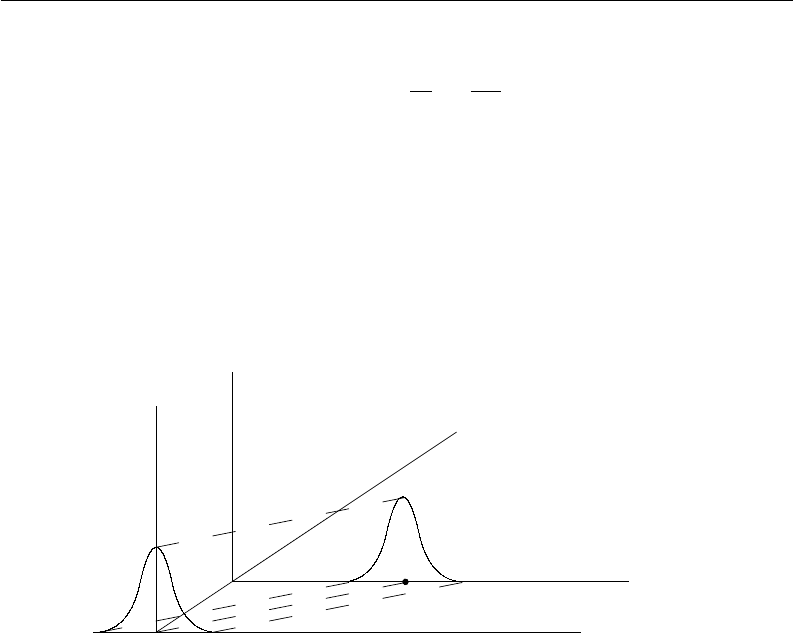
6.2.11. Solve the following problem in the domain −∞ < x < ∞, t ≥ 0 :

= a

, u(x,0) = f (x), u

(x,0) = −a f

(x),

where f is a smooth function (see ﬁg. 6.2.1).

u(x,t)

= f (

x −at)

Figure

6.2.1.

Method of separation of variables

Sturm-Liouville problem. Consider the following boundary value problem L

−(k(x)y

(x))

+ q(x)y(x) = λρ(x)y(x), 0 ≤x ≤l,

(0) + hy(0) = H

(l) + Hy(l) = 0,

which is called the Sturm-Liouville problem. Here λ is the spectral parameter, k,q, ρ

are real-valued functions, and h

,h, H

,H are real numbers. We assume that ρ(x),k(x) ∈

[0,l] (i.e. ρ(x),k(x),ρ

(x),k

(x) are absolutely continuous functions), q(x) ∈ L(0,l) ,

ρ(x) > 0, k(x) > 0 , and |h

|+ |h| > 0 , |H

|+ |H| > 0 . We are interested in non-trivial

solutions of the boundary value problem L .

The values of the parameter λ for which L has nonzero solutions are called eigenval-

ues, and the corresponding nontrivial solutions are called eigenfunctions.

It is known that L has a countable set of eigenvalues {λ

}

n≥0

, and λ

= O(n

) as

n → ∞ . For each of these eigenvalues λ

there exists only one eigenfunction (up to a

234 G.

Freiling and V. Yurko

multiplicativ

e constant) y

(x) . The set of eigenfunctions {y

(x)}

n≥0

form a complete and

orthonormal system in L

[0,l] with the weight r(x) , i.e.:

ρ(x)y

(x)y

(x)dx =

0, n 6= m,

1, n = m,

If f (x) is a twice continuously differentiable function satisfying boundary conditions, then

f (x) can be expanded into the uniformly convergent series:

f (x) =

∞

∑

n=1

(x),

where

ρ(x) f (x)y

(x)dx.

Note that for the case h

6= 0 , these facts were proved in section 2.2 (see Theorem 2.2.8).

Other cases can be treated similarly.

6.2.11. Find eigenvalues and eigenfunctions of the boundary value problems for the

equation y

+ λy = 0 ( 0 < x < l ) with the following boundary conditions:

1. y(0) = y(l) = 0;

2. y

(0) = y

(l) = 0;

3. y(0) = y

(l) = 0;

4. y

(0) = y(l) = 0;

5. y

(0) = y

(l) + hy(l) = 0.

Solution of Problem 1. Let λ = ρ

. The general solution of the equation y

+ λy = 0

has the form

y(x) = C

sinρx

cosρx.

Using

the

boundary condition y(0) = 0, we get C

= 0. The second boundary condition

y(l) = 0 gives us the equation that must be satisﬁed by the eigenvalues:

sinρl

= 0.

Hence,

the

eigenvalues and the eigenfunctions of Problem 1 have the form

nπ

, y

(x)

= sin

x, n = 1,2,

6.2.12. Find eigenvalues and eigenfunctions of the following boundary value problems

(0 < x < l) :

1. −y

+ γy = λy, y(0) = y(l) = 0;

Exercises 235

2. −y

+ γy = λy, y

(0) = y

(l)

= 0;

3. −y

+ γy = λy, y(0) = y

(l) = 0;

4. −y

+ ηy

+ γy = λy, y(0) = y(l) = 0.

Solution of Problem 4. The replacement

y(x) = exp

ηx

Y (x)

yields

(x)

= e

ηx

(x)

Y (x)

(x)

= e

ηx

(x)

+ ηY

(x)

Y (x)

and

consequently

(x) + µY (x) = 0, Y (0) = Y (l) = 0,

where µ = λ −

−γ. The

eigen

values and the eigenfunctions of this boundary value

problem are

nπ

, Y

(x)

= sin

x, n ≥1

(see

Problem

6.2.11). Therefore, the eigenvalues and the eigenfunctions of Problem 4 have

the form

nπ

+ γ, y

(x)

= e

ηx

sin

nπ

x, n ≥1.

Let

brieﬂy present the scheme of the method of separation of variables for solving

the mixed problem for a vibrating string. Consider the following mixed problem for the

equation

ρ(x)u

= (k(x)u

)

−q(x)u, 0 ≤ x ≤l, t ≥0 (6.2.1)

with the initial conditions

u(x,0) = ϕ(x), u

(x,0) = ψ(x) (6.2.2)

and with the boundary conditions

+ hu)|

x=0

= (H

+ Hu)|

x=l

= 0. (6.2.3)

First we consider the following auxiliary problem. We will seek nontrivial (i.e. not

identically zero) particular solutions of equation (6.2.1) such that they satisfy the boundary

conditions (6.2.3) and admit separation of variables, i.e. they have the form

u(x,t) = T (t)y(x). (6.2.4)

Substituting (6.2.4) into (6.2.1) and (6.2.3), we get the Sturm-Liouville problem L for the

function y(x), and the equation T

(t) + λT (t) = 0 for the function T (t).

236 G.

Freiling and V. Yurko

Let λ

(x) (n = 0

,1, 2,. ..) be the eigenvalues and the eigenfunctions of the problem

L . Then the functions

(x,t) =

cos

t + B

sin

√

(x)

.2.5)

satisfy the equation (6.2.1) and the boundary conditions (6.2.3) for any A

and B

. The

solutions of the form (6.2.5) are called standing waves (normal modes of vibrations).

We will seek the solution of the mixed problem (6.2.1)-(6.2.3) by superposition of

standing waves (6.2.5):

u(x,t) =

∞

∑

n=0

cos

t + B

sin

√

(x). (6.2.6)

we use the initial conditions (6.2.2) for ﬁnding the coefﬁcients A

and B

. For this

purpose we substitute (6.2.6) into (6.2.2) and calculate

ϕ(x) =

∞

∑

n=0

(x), ψ(x) =

∞

∑

n=0

(x).

Then the coefﬁcients A

and B

are given by the formulae

ρ(x)ϕ(x)y

(x)dx, B

ρ(x)ψ(x)y

(x)dx.

6.2.13. Solve the following problems of oscillations of a homogeneous string (0 < x <

l) with ﬁxed end-points if the initial displacement u(x,0) and the initial velocities u

(x,0)

have the form:

1. u(x,0) = A sin

πx

, u

(x,0)

= 0;

2. u

(x,0) =

x(l −x), u

(x,0)

= 0;

3. u

(x,0) =

(0 ≤ x ≤C), u(x,0)

(l −x)

l −C

(C ≤ x ≤l),

(x,0)

= 0;

4. u

(x,0) = 0, u

(x,0) = v

−const;

5. u(x,0) = 0,

(x,0) = v

(α ≤ x ≤β), u

(x,0) = 0 (x /∈ [α, β]);

6. u(x,0) = 0, u

(x,0) = sin

2π

Exercises 237

Solution of

Problem 1. We have to solve the following mixed problem

= a

, 0 < x < l, t > 0,

|x=0

= u

|x=l

= 0,

|t=0

= A sin

x, u

t|t=0

= 0.

This

problem

is a particular case of the mixed problem (2.2.1)-(2.2.3) when ϕ(x) =

Asin

x , ψ(x)

= 0

. According to (2.2.17)-(2.2.18) the solution has the form

u(x,t) =

∞

∑

n=1

sin

anπ

t + B

cos

anπ

sin

nπ

x ,

where

= 0, B

Asin

x sin

nπ

Clearly, B

= A and B

= 0 for n ≥2, and consequently,

u(x,t) = A cos

aπ

t sin

x .

6.2.14. Solv

the following problems of oscillations of a homogeneous string (0 < x <

l) with free end-points if the initial displacement u(x,0) and the initial velocities u

(x,0)

have the form:

1. u(x,0) = 1, u

(x,0) = 0;

2. u(x,0) = x, u

(x,0) = 1;

3. u(x,0) = cos

πx

, u

(x,0)

= 0;

4. u

(x,0) = 0, u

(x,0) = v

(α ≤ x ≤β), u

(x,0) = 0 (x /∈ [α, β]).

Solution of Problem 2. We have to solve the following mixed problem

= a

, 0 < x < l, t > 0,

x|x=0

= u

x|x=l

= 0,

|t=0

= x, u

t|t=0

= 1.

First we seek nontrivial particular solutions of the equation of the form u(x,t) = Y (x)T (t),

which satisfy the boundary conditions. Repeating the arguments from section 2.2 we obtain

for the function T (t) the ordinary differential equation

T (t) + a

λT (t) = 0,

238 G.

Freiling and V. Yurko

and for

the function Y (x) we get the Sturm-Liouville boundary value problem

(x) + λY (x) = 0, Y

(0) = Y

(l) = 0.

Here λ is the spectral parameter. The eigenvalues and the eigenfunctions of this boundary

value problem are

nπ

, Y

(x)

= cos

x, n ≥0.

The

corresponding

equations

(t) + a

(t) = 0, ,n ≥0,

have the general solutions

(t) = A

t + B

, T

(t) = A

sin

anπ

t + B

cos

anπ

t, n ≥1,

where A

and B

are

arbitrary

constants. Hence,

(x,t) = A

t + B

(x,t) =

sin

anπ

t + B

cos

anπ

cos

nπ

x, n ≥1.

seek the solution of the mixed problem of the form

u(x,t) = A

t + B

∞

∑

n=1

sin

anπ

t + B

cos

anπ

cos

nπ

x ,

and

ﬁnd A

and B

from the initial conditions:

x = B

∞

∑

n=1

cos

nπ

x ,

1 = A

∞

∑

n=1

anπ

cos

nπ

x ,

and

hence

x =

, A

x = 1

x cos

nπ

x =

(

(−1

)

−1), n ≥1,

anπ

cos

nπ

x = 0, n ≥1.

This yields

u(x,t) = t +

∞

∑

n=1

((−1)

−1)cos

anπ

t cos

nπ

x .

6.2.15. Solv

the following problems of oscillations of a homogeneous string (0 < x <

l) if the initial and boundary conditions have the form:

Exercises 239

1. u(x,0) = x, u

(

x,0) = sin

x, u(0,t)

= u

(l,t)

= 0;

2. u(x,0) = cos

x, u

(x,0)

= 0

, u

(0,t) = u(l,t) = 0;

3. u(x,0) = 0, u

(x,0) = 1, u

(0,t) = u

(l,t) + hu(l,t) = 0;

4. u(x,0) = sin

3π

x, u

(x,0)

= cos

x, u(0,t)

= u

(l,t)

= 0.

Solution of Problem 2. We have to solve the following mixed problem

= a

, 0 < x < l, t > 0,

x|x=0

= u

|x=l

= 0,

|t=0

= cos

x, u

t|t=0

= 0.

First

seek nontrivial particular solutions of the equation of the form u(x,t) = Y (x)T (t),

which satisfy the boundary conditions. Repeating the arguments from section 2.2 we obtain

for the function T (t) the ordinary differential equation

T (t) + a

λT (t) = 0,

and for the function Y(x) we get the Sturm-Liouville boundary value problem

(x) + λY (x) = 0, Y

(0) = Y (l) = 0.

The eigenvalues and the eigenfunctions of this boundary value problem are

(2n + 1)π

, Y

(x)

= cos

n + 1)π

x, n ≥0.

The

corresponding

equations

(t) + a

(t) = 0, ,n ≥0,

have the general solutions

(t) = A

sin

a(2n + 1)π

t + B

cos

a(2n + 1)π

t, n ≥0,

where A

and B

are

arbitrary

constants. Hence,

(x,t) =

sin

a(2n + 1)π

t + B

cos

a(2n + 1)π

cos

(2n + 1)π

x .

seek the solution of the mixed problem of the form

u(x,t) =

∞

∑

n=0

sin

a(2n + 1)π

t + B

cos

a(2n + 1)π

cos

(2n + 1)π

x ,

240 G.

Freiling and V. Yurko

and we

ﬁnd A

and B

from the initial conditions:

cos

x =

∞

∑

n=0

cos

(2n + 1)π

x ,

0 =

∞

∑

n=0

a(2n + 1)π

cos

(2n + 1)π

x ,

and

hence

= 1

, B

= 0, n ≥ 1, A

= 0, n ≥0.

This yields

u(x,t) = cos

aπ

t cos

x .

6.2.16. Solv

the following mixed problems applying the method of separation of vari-

ables:

1. u

= u

−4u, 0 < x < 1,

u(x,0) = x

−x, u

(x,0) = 0, u(0,t) = u(1,t) = 0;

2. u

= u

+ u, 0 < x < π,

u(x,0) = 0, u

(x,0) = 1, u

(0,t) = u

(π,t) = 0;

3. u

= t

, (α > −1), 0 < x < l,

u(x,0) = ϕ(x), u

(x,0) = 0, u(0,t) = u(l,t) = 0;

4. u

+ 2u

= u

−u, 0 < x < π,

u(x,0) = πx

−x

, u

(x,0) = 0, u(0,t) = u(π,t) = 0;

5. u

+ 2u

= u

−u, 0 < x < π,

u(x,0) = 0, u

(x,0) = x, u

(0,t) = u(π,t) = 0;

6. u

= a

(xu

)

, 0 < x < l,

u(x,0) = ϕ(x), u

(x,0) = 0, |u(0,t)| < ∞, u(l,t) = 0.

Solution of Problem 1. First we seek nontrivial particular solutions of the equation of

the form u(x,t) = Y (x)T (t), which satisfy the boundary conditions. We obtain for the

function T (t) the differential equation

T (t) + λT (t) = 0,

and for the function Y(x) we get the Sturm-Liouville boundary value problem

(x) + (λ −4)Y (x) = 0, Y (0) = Y (l) = 0.

The eigenvalues and the eigenfunctions of this boundary value problem are

= (nπ)

+ 4, Y

(x) = sin nπx, n ≥1.

Exercises 241

The corresponding

equations

(t) + λ

(t) = 0, n ≥ 1,

have the general solutions

(t) = A

cosρ

t + B

sin

, n ≥1,

where A

and B

are

arbitrary

constants, and ρ

(nπ)

+ 4 .

Hence,

(x,t)

cosρ

t + B

sin

sinnπx, n ≥ 1.

seek the solution of the mixed problem of the form

u(x,t) =

∞

∑

n=1

cosρ

t + B

sin

sinnπx,

and

ﬁnd A

and B

from the initial conditions:

−x =

∞

∑

n=1

sinnπx, 0 =

∞

∑

n=1

sinnπx,

and hence

= 2

−x)sinnπx dx =

((−1)

−1), B

= 0, n ≥1.

This

yields

(x,t) =

∞

∑

n=1

(

(−1

)

−1)cos(

+ 4t)sin nπx.

Solution

Problem 5. First we seek nontrivial particular solutions of the equation of

the form u(x,t) = Y (x)T (t), which satisfy the boundary conditions. We obtain for the

function T (t) the differential equation

T (t) + 2

T (t) + λT (t) = 0,

and for the function Y(x) we get the Sturm-Liouville boundary value problem

(x) + (λ −1)Y (x) = 0, Y

(0) = Y (π) = 0.

The eigenvalues and the eigenfunctions of this boundary value problem are

n +

+ 1, Y

(x)

= cos

n +

x, n ≥0.

The

corresponding

equations

(t) +

(t) + λ

(t) = 0, n ≥ 1,